RL Long Tail: Mid-Batch Parallel Shape Switching
On four A100s with no NVLink, switching an RL rollout from DP4 to TP4 once the long tail remains is 1.31 times slower than staying on DP2×TP2. The two-GPU custom all-reduce keeps the mixed shape ahead in both the crowded phase and the sparse phase, and one switch costs at least 19 seconds, more than it can save.
Training a reasoning model with reinforcement learning starts each step by letting the current policy write an answer to every problem in a batch. That step is the rollout. Answer lengths spread widely. Most finish in a few thousand tokens. A few write until the length cap. The first half of the batch keeps every GPU full. The second half is a handful of long requests, and the batch cannot finish until they do. A natural guess is to serve the crowded half in a high-throughput shape, then switch to a low-latency shape for the tail. This article tests that guess on an ordinary four-GPU PCIe machine. It does not hold. The reason is more useful than the guess.
Three ways to place the same four GPUs
An 8B dense model in bf16 is about 16 GB, and one 40 GB A100 holds it. Data parallelism, DP, puts a full copy on every GPU and serves a separate slice of the requests. Four GPUs are DP4, four queues and no communication between them. Tensor parallelism, TP, splits each layer’s weight matrices across GPUs, the Megatron-LM cut (Shoeybi et al. 2019). After the layer, an all-reduce adds the partial results. Four GPUs as one engine are TP4. Between them is a mixed shape, DP2×TP2, two TP2 engines of two GPUs each.
The tradeoff sits in decode. Each step emits one token per request in the batch, and it has to read the whole weight tensor plus the KV cache of the context so far. A100 memory bandwidth is about 1.555 TB/s, so reading 16 GB of weights is about 10 ms. That is the order of a single-GPU, single-request token time. TP cuts the weights into N pieces, so each GPU reads 1/N, and the token time falls. The cost is two all-reduces per layer. This Llama-shaped 8B model has 32 layers, so a step does 64 all-reduces. The message is the batch size times hidden size 4096 times 2 bytes. At 16 requests that is 128 KiB. DP has no communication, and each GPU reads every weight, so a single request is slower. Its advantage is throughput, because four engines can each grow their own batch. The usual rule of thumb is that DP wins when many requests are in flight, and TP wins when few remain.
In a batch of 16 requests at about ten thousand tokens of context, each request’s KV cache is about 128 KiB per token: 32 layers, 8 KV heads, head dimension 128, key and value, bf16. The batch is about 20 GB, larger than the weights. KV bytes per GPU depend on how many requests that GPU serves. At the same total number of requests in flight, TP4 and two TP2 engines read the same KV bytes per GPU. Only the weight read differs.
Which path the all-reduce takes
Whether the all-reduce is cheap depends on the path. NCCL’s ring cuts the data into chunks and passes them 2(N−1) times around N GPUs (NVIDIA, NCCL). It is bandwidth-optimal for large messages, and a small message pays tens of microseconds of protocol. Decode all-reduces are many small messages, so vLLM (Kwon et al. 2023) ships its own custom all-reduce. GPUs map each other’s buffers with CUDA IPC and reduce in one kernel over peer-to-peer reads, either one-shot or two-shot, and skip the NCCL protocol (vLLM custom all-reduce).
The implementation turns on only for a full NVLink mesh, or for exactly two PCIe-only GPUs. With more than two PCIe-only GPUs, vLLM logs that custom all-reduce is disabled and falls back to NCCL. On this machine two A100s share a PCIe switch, and the two switches meet at the CPU host bridge. A measured 128 KiB all-reduce is about 20.6 µs on the two-GPU custom path and about 93.4 µs on the four-GPU NCCL path, more than four times slower. Times 64 per step, that is about 1.3 ms against about 6 ms, a first-order term inside a decode step of ten-plus milliseconds.
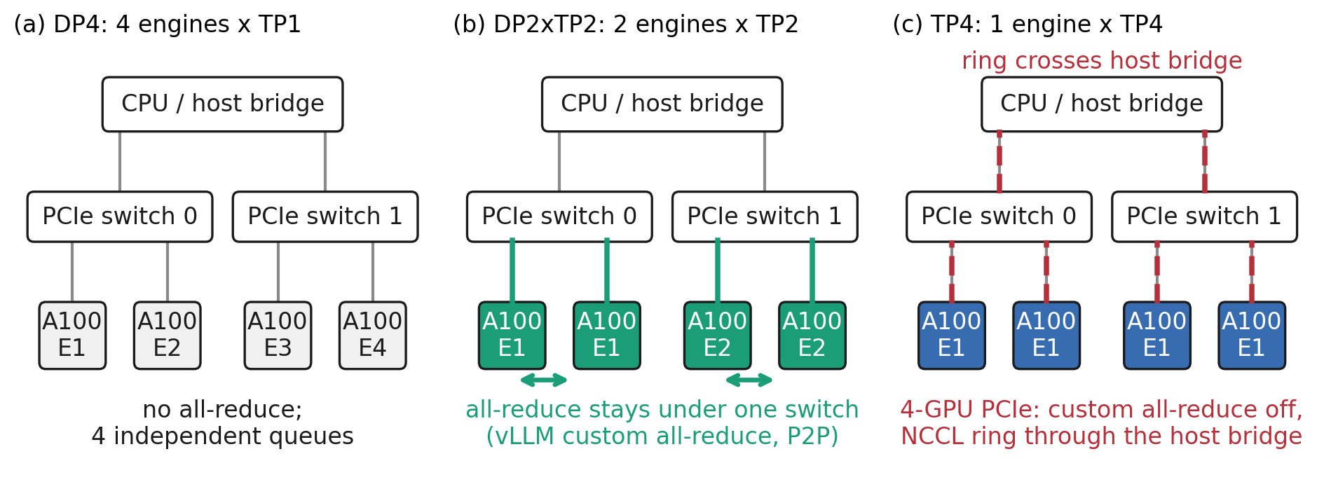
Going from TP2 to TP4 is not one more GPU on the same path. It is a different communication implementation and a longer physical route.
The long tail, and systems that already reconfigure
RL stacks usually run the rollout on an inference engine. HybridFlow, verl, alternates generation and training on the same GPUs (Sheng et al. 2024). Reasoning training makes rollouts long. DeepSeek-R1 reports that answer length keeps growing during training (DeepSeek-AI 2025). Kimi k1.5 cuts over-long trajectories and resumes them across iterations (Kimi Team 2025). The batch here has the same shape. Problems come from MATH-500 (Lightman et al. 2023), itself drawn from MATH (Hendrycks et al. 2021). The median output is about 2400 tokens, the 90th percentile about 9800, and about 3% to 4% of requests write to the 16K cap.
Systems already change deployment shape at runtime. Llumnix migrates live requests across instances (Sun et al. 2024). DistServe (Zhong et al. 2024) and Splitwise (Patel et al. 2024) put prefill and decode on different GPUs. NVIDIA Dynamo decides per request whether to split them, from the effective input length and the prefill load (NVIDIA Dynamo). That choice already switches at zero migration cost. TP degree has no in-process switch. The available pattern is one resident engine per shape. An idle engine enters vLLM sleep mode, swaps weights to host memory, frees the KV pool, and wakes in a few seconds (vLLM sleep mode). A request that must change shape is cancelled and resubmitted on the target engine, with the problem plus the tokens already written as the new prompt. The cost is a prefill of that context.
TL;DR
The question is whether a long-tailed RL rollout finishes sooner if the parallel shape changes mid-batch. The guess is that DP4 is the high-throughput first half and TP4 is the fast-per-token second half, so one switch takes both.
On four A100s in two PCIe-switch pairs, the switch point chosen from an offline profile is 1.31 times slower than static DP2×TP2. DP2×TP2 loses neither phase. TP4 is only 0% to 11% faster per token than TP2 in the tail. One switch pauses for at least 19 seconds.
The makespan of a long-tail batch is about the length cap times the lifetime average token time of the longest request. On a PCIe-only machine, that time is set by whether the all-reduce can stay under one switch.
The hypothesis
There is a threshold n*, the number of requests still in flight. Run DP4 until only n* requests remain, move them to TP4, and finish. The makespan, the time of the last completion, should beat the best of DP4, TP4, DP2×TP2, and a length-based spatial split by at least 15%. The paired 95% confidence interval should exclude zero. Every switch and recompute cost counts. The 15% bar is there so a tuning delta does not pass.
The guess looked plausible from a single-request microbenchmark and an order-of-magnitude estimate. At one request and 1K of context, four-GPU TP4 is about 2.4 times faster per token than one GPU, and at a loose latency target DP4’s capacity is about 2.5 times TP4. A two-phase closed form says why both sides have to be large. When the two phases each take half the time, picking the best shape per phase beats the best static choice by 15% only if each side leads by about 36% in the symmetric case. A large lead on one side and a small lead on the other gives almost nothing. Putting the curves into a fluid simulation of 128 requests with log-normal lengths, the most favorable cell is four GPUs, a wide length spread, and a 16K cap. The median gain there is 5.9%, and the maximum is 27%. The estimate’s weakness was written down at the time. The curves are from 1K of context, a long context reads more KV per step, and the comparison is only TP4 against DP4. The mixed shape is not in it.
How it was measured
The machine is one node, four A100-PCIe 40 GB GPUs, two per PCIe switch, the switches joined by the host bridge, and no NVLink. The software is vLLM 0.25.1, PyTorch 2.11, CUDA 13.0, bf16, with prefix caching, chunked prefill, and CUDA graphs at their defaults. The model is DeepSeek-R1-Distill-Llama-8B. The workload is the first 256 problems of MATH-500 after a fixed shuffle, with the R1 math prompt, temperature 0.6, top_p 0.95, and a cap of 16384 tokens, ending on EOS. All 256 requests arrive at time zero. The other 244 problems are only for the offline profile. Three seeds. Within a seed every configuration sees the same problems and the same per-request sampling seed. Statistics are paired by seed. The 95% interval uses a t distribution with 2 degrees of freedom.
Five families. DP4, TP4, and DP2×TP2 are static. SPLIT@L is a spatial split. New requests enter two TP1 engines on two GPUs, and a request whose output passes L tokens moves to a TP2 engine on the other two GPUs. L is 2048, 4096, or 8192. DYN@n is the dynamic policy. Start on DP4. When unfinished requests fall to n, cancel them, wait for the four TP1 engines to drain, put those engines to sleep, wake a prewarmed TP4 engine, and resubmit the remainder with the tokens already generated. n is 8, 16, 32, 64, or 128. n=32 is the point an offline predictor, looking only at the profile batch, picked before the measurement batch ran. That point was registered in advance. Every configuration runs on the same resident engines, and unused engines are in L1 sleep. Standalone DP4 and TP4, not coresident and not using sleep, differ from the coresident versions by 1.0% to 1.2%. Output token count and answer accuracy are controls, so an early stop cannot fake a speedup.
One measurement trap is worth stating. transformers 5.x loads this model’s tokenizer as a Llama-2-style class and eats spaces on encode. The server tokenizer in the same vLLM image does the same. The model still answers, and nothing errors. The first smoke run was discarded. The reported runs encode with tokenizer.json directly and check that decoding returns the original text.
The mixed shape wins both phases
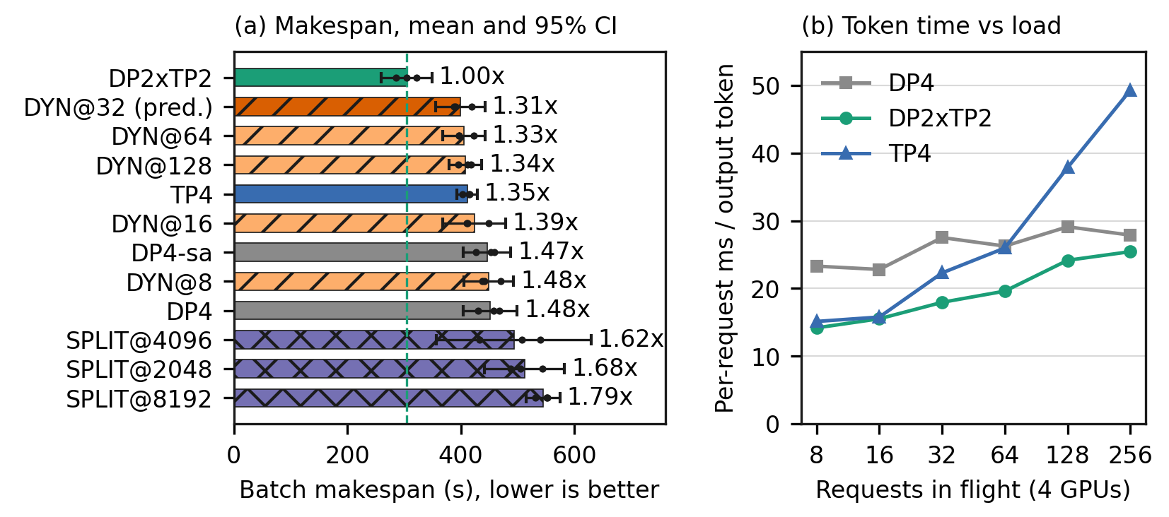
DP2×TP2 finishes in 304 seconds. The preregistered DYN@32 takes 399 seconds, 1.31 times DP2×TP2. The paired difference is +94.9 seconds, 95% interval [+8.9, +181.0], and it excludes zero. TP4 is 411 seconds. DP4 is 452 seconds. The three spatial splits are 493 to 545 seconds. A one-seed standalone TP4 at 415 seconds is not on the figure. The dynamic policy is 11.6% faster than DP4, interval [0.9%, 22.2%], and its gap to TP4 is inside the noise. The reversal between DP4 and TP4 is real, and a switch collects about 10% of it. A mixed shape that wins both phases takes that gain away. The paired difference in output tokens is +25K, inside the seed noise (standard deviation 23K). The accuracy difference is −0.9 percentage points, under twice that noise.
The ordering is the request that finishes last. In every configuration and every seed, that request hits the 16384 cap. Makespan is almost 16384 times its lifetime average token time. On DP2×TP2 that average is 18.5 ms, which is 303 seconds. On TP4 it is 24.9 ms, which is 408 seconds. Both match the measurement. A long request lives through a crowded phase, hundreds of requests together, and then a sparse phase of a few requests. Makespan is the weighted average of those two phases, not the tail speed alone.
Figure 2(b) splits the weight. The horizontal axis is requests in flight on the four GPUs. The vertical axis is the token time a request actually sees, engine concurrency times the sample interval divided by tokens that engine emitted, median across the three seeds. In the crowded phase TP4 is worst. At 256 in flight it is about 49 ms per token, twice DP2×TP2 at about 25 ms, because one TP4 engine pushes 256 requests’ all-reduce messages, about 2 MiB, across the host bridge, and it has one scheduler. DP4 is close to DP2×TP2 while crowded, and it is the slowest in the sparse phase, about 23 ms, because every GPU reads the full weights. At 8 to 16 in flight, TP4 and DP2×TP2 nearly meet. At 16 they are 15.8 ms against 15.5 ms. Read per engine instead, TP4 at 16 in flight is 15.1 ms and a TP2 engine at 8 in flight is 16.9 ms, so TP4 is 11% faster. That is the reading most favorable to TP4. Neither reading has the 2.4 times the desk estimate used.
The same order-of-magnitude split explains it. At the same total number of requests in flight, TP4 and two TP2 engines read the same KV bytes per GPU. The weights differ. TP2 reads 8 GB per GPU per step, about 5.1 ms. TP4 reads 4 GB, about 2.6 ms, and saves about 2.6 ms. On the other side, 16 requests mean 64 all-reduces of 128 KiB. The two-GPU custom path is about 1 ms. The four-GPU NCCL path is about 6 ms. The two terms are the same size and opposite in sign, so the tail advantage lands between zero and about ten percent. Every shape’s step time is 2 to 5 ms above a pure bandwidth model, and TP4 is the furthest above it. This article does not break that remainder into sampling, scheduling, and the all-reduce. The conclusion depends on custom all-reduce being off for four GPUs, and on the two groups crossing a host bridge. On a full NVLink mesh, TP4 would still use the custom path or a faster one, and this arithmetic would change.
What one switch costs
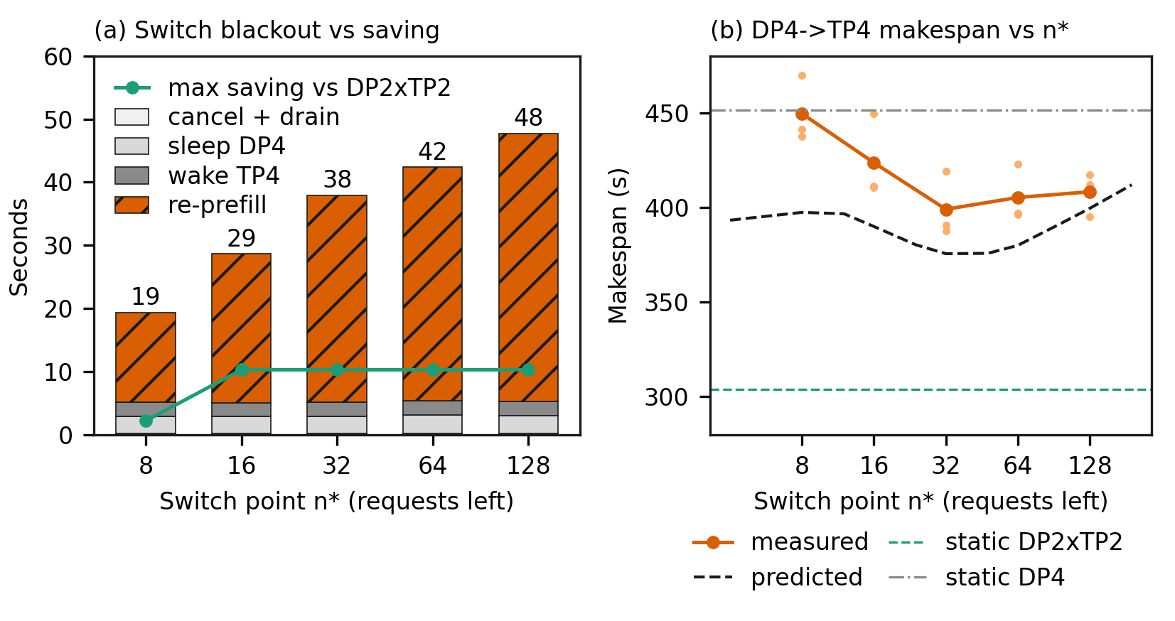
Cancel and drain are about 0.2 seconds. Sleeping the four TP1 engines is about 2.7 seconds, a copy of four 16 GB weight sets back to pinned host memory. Waking TP4 is about 2.2 seconds. Then comes the re-prefill, from resubmit until every migrated request has its first new token. The fixed part stays at 5.0 to 5.4 seconds. Re-prefill grows from 14 seconds at n*=8 to 43 seconds at n*=128. The whole pause is 19 to 48 seconds. Re-prefill dominates for a one-line reason. At n*=32, 32 migrated requests carry about 8K of context each, about 257,000 tokens. TP4 prefill is only about 7.8K tokens per second. 32 times 8K divided by 7.8K is about 33 seconds, and the measurement is 32.8 seconds. The prefill rate itself is the less intuitive part. Four-GPU TP4 is slower than one GPU running TP1, about 11.2K tokens per second, because prefill all-reduces are large and the host-bridge bandwidth is the limit. The same topology fact both shrinks TP4’s tail gain and raises the cost of switching to it.
The green line is an upper bound on the saving against DP2×TP2. It is analysis, not a measurement. Take DP2×TP2’s own tail duration and multiply by the 11% per-step advantage that is the most favorable reading for TP4. The tail while at most 8 requests remain averages 19.9 seconds, so the bound is about 2.2 seconds. At most 16 requests, the tail is 93.5 seconds and the bound is about 10.3 seconds. Above 16 in flight, TP4 is slower than DP2×TP2, so switching earlier only loses, and the bound caps near 10 seconds. The measured pause starts from DP4. Starting from DP2×TP2 would sleep two TP2 engines. The fixed part is the same order, and the re-prefill follows the migrated context, the same order. The smallest pause, 19 seconds, is about twice the most the switch can save. No switch point makes a one-time move off the best static shape pay for itself.
Figure 3(b) is the predictor. The solid line is measured DYN@n makespan. The dashed line is the offline predictor, using only the profile batch’s DP4 and TP4 curves, a switch probe, and the prefill rate. It picks n*=32, which is also the measured best point. That agreement carries little information. The points at 32, 64, and 128 differ by 2.3%, less than the seed standard deviation of one configuration, 11 to 18 seconds. The absolute prediction is systematically 6% to 16% optimistic. The bias sits in the DP phase. Static DP4 is underestimated by 15.7%, TP4 by 1.4%. Feeding the real output lengths does not fix it, at −7.2%, because the model looks up throughput by per-engine concurrency and does not represent the imbalance after round-robin assignment. The four DP engines’ last completions differ by 90 to 127 seconds. The switch-cost model, a fixed 5.5 seconds plus context divided by the prefill rate, errs by −2% to −6%. An offline profile can rank the switch point and can price the switch. What it misses is the tail of the DP shape.
Why the conjecture does not hold
The hypothesis fails in its own experiment, and what fails is the premise. A 2.4 times faster TP4 token in the tail does not hold at long context and a dozen requests in flight. The measurement is zero to about ten percent. Without that premise, the two-phase relation never gets the roughly 36% lead it needs on both sides. The crowded-phase winner is not DP4. It is DP2×TP2. A static mixed shape wins both phases, and any single switch that pays a recompute can only be slower. The first-round estimate that picked the scenario compared only TP-N with DP-N. It left the mixed shape out, and the mixed shape is what won.
A few gaps remain. Three seeds leave a wide interval. DYN@32’s makespan interval is [356, 442] seconds. The paired difference against DP2×TP2 still excludes zero, so the direction is stable. A network job that uses no GPU was running on the same node, and its NIC shares a PCIe switch with two of the GPUs. Host CPU was 5.4% busy over the run. That interference was not removed. If it matters, it is more likely to hurt the cross-switch TP4 path, which is the direction against the dynamic policy, and it is not large enough to explain a 95 second gap. One model, one length cap, and one topology were measured. A shorter cap makes the tail shorter and gives TP4 less time to help, which is worse for switching, and it was not measured. Splitting or fusing prefill and decode was not measured. Per-request choices of that kind already exist in shipping systems at zero switch cost, and this article does not judge their gain.
What sets the makespan
The makespan of a long-tail batch is about the length cap times the lifetime average token time of the longest request. In every configuration and every seed the last request hits the 16K cap. 18.5 ms times 16384 is 303 seconds, and 24.9 ms times 16384 is 408 seconds, within 1% of the measured makespan. What to optimize is a shape’s weighted behavior in the crowded phase and the sparse phase, not its peak tail speed. This holds when output length has a hard cap and some requests hit it. About 3% to 4% of this batch do.
On a PCIe-only multi-GPU node, the best parallel shape is set by the board topology. A concurrency-1 microbenchmark says the opposite. vLLM 0.25.1 enables custom all-reduce only for two PCIe-only GPUs. With four A100s on two switches, TP4 falls back to NCCL across the host bridge. In the tail it is only 0% to 11% faster per token than TP2. In the crowded phase its aggregate throughput is about half of DP2×TP2, and its prefill is slower than one GPU. DP2×TP2, with each TP pair under one switch, wins both phases. Its makespan is 26% shorter than TP4 and 33% shorter than DP4. This is for no NVLink, two GPUs per switch, an 8B dense model, and contexts of thousands to tens of thousands of tokens. A full NVLink mesh is a different machine.
A dynamic choice between two shapes pays only when the winner of each phase leads by about a third. When the two phases take similar time and the switch is free, each side needs about a 36% lead before phase-by-phase selection beats the best static choice by 15%. A large lead on one side and a small lead on the other goes to about zero. Charging the switch only raises the bar.
The pause of moving a live request across parallel shapes is a fixed few seconds plus the migrated context divided by the target shape’s prefill rate. The saving cannot exceed the target’s per-step advantage times the remaining tail. Both can be computed offline before the switch. Here the fixed part is 5.0 to 5.4 seconds, sleep 2.7 and wake 2.2. Re-prefill is 70% to 90% of the pause. The cost model errs by −2% to −6%. The smallest pause is 19 seconds against a maximum saving of about 10 seconds. This assumes a prewarmed engine per shape, continuation by recomputing the tokens already written, and one PCIe node. A primitive that moves KV across layouts would shrink the recompute term. None was available to measure.
A comparison of parallel shapes has to include the mixed shape. TP-N against DP-N shows a real reversal. The switch is 11.6% faster than DP4, and the interval excludes zero. That reversal does not change the deployment, because DP2×TP2 is faster than both ends. This applies when the GPU count allows a mix, four or more, and the topology groups the GPUs into better-connected pairs.
These numbers cover one machine of four A100-PCIe 40 GB GPUs, two PCIe-switch pairs, no NVLink, one 8B dense reasoning model, one math-rollout batch, a 16K cap, and three seeds. They do not say that a structural dynamic switch is never worth it. They do not say DP2×TP2 dominates on NVLink, on another PCIe topology, or on a larger model. They say nothing about a prefill-decode phase reversal. A −0.9 percentage point accuracy gap is not evidence that the dynamic switch hurts or helps answer quality.
The mixed shape already covers both phases
DP2×TP2 is ahead while the batch is crowded and it is not behind in the tail. Moving to TP4 for the tail pays at least 19 seconds to save at most about 10. On this board, the shape that keeps each all-reduce under one switch is the one to run for the whole batch.
Related analysis
Where Communicator Rebuild Actually Costs measures the NCCL cost of rebuilding a communicator when the parallel shape changes. When the shapes can be listed in advance, a prewarmed pool already takes that cost off the critical path.
Hybrid PD Handoff: Does Waiting by Component Beat Waiting by Layer? asks, once prefill and decode are already on different GPUs, whether the handoff should wait per component or per layer. On that model, the extra gain of waiting per component stays near zero.
在四张没有 NVLink 的 A100 上,rollout 长尾里从 DP4 切到 TP4,比一直跑 DP2×TP2 慢,完成时间是它的 1.31 倍。两卡 custom all-reduce 让混合形态在拥挤段和稀疏段都赢。一次切换最少停 19 秒,大于任何能省下的时间。
强化学习训练推理模型时,每一步先让当前策略对一批题目各写一段回答。这一步叫 rollout。回答长度很散。多数几千 token 就结束,少数一直写到长度上限。一批的前半程几百个请求同时在跑,GPU 是满的。后半程只剩几个长请求,整批却要等它们结束。一个自然的想法是前半程用吞吐高的形态,后半程换成单请求更快的形态。这篇文章在一台普通的 PCIe 四卡机器上检验这个想法。它不成立。否定它的原因比这个想法更值得记住。
同一组 GPU 的三种摆法
8B 的稠密模型用 bf16 大约 16 GB,一张 40 GB 的 A100 放得下。数据并行(DP)是每张卡放一份完整模型,各自服务一部分请求。四张卡就是 DP4,四个互不通信的队列。张量并行(TP)把每一层的权重矩阵切到多张卡上,这是 Megatron-LM 的切法(Shoeybi et al. 2019)。每层算完做一次 all-reduce。四张卡合成一个引擎就是 TP4。中间还有混合形态,例如 DP2×TP2,两个 TP2 引擎各占两张卡。
取舍出在 decode。每一步为批里每个请求生成一个 token,要把全部权重读一遍,还要读每个请求已有上下文的 KV cache。A100 显存带宽约 1.555 TB/s,读一遍 16 GB 权重大约 10 ms,这是单卡单请求每 token 时间的量级。TP 把权重切成 N 片,每卡每步只读 1/N,单请求每 token 时间下降。代价是每层两次 all-reduce。这个 Llama 结构的 8B 模型有 32 层,每步 64 次。消息大小是批大小乘隐藏维 4096 乘 2 字节。16 个请求时每次 128 KiB。DP 没有通信,但每张卡都要读全部权重,单请求更慢。它的优势是吞吐,四个引擎可以各自把批做大。常见的经验是请求多时 DP 吞吐高,请求少时 TP 延迟低。
16 个请求、上下文约一万 token 时,每个请求的 KV cache 约 128 KiB 每 token。32 层、8 个 KV 头、头维 128、键和值、bf16。合计约 20 GB,比权重还大。总在制请求数相同时,TP4 和两个 TP2 引擎每张卡读的 KV 字节数一样。不一样的只有权重。
all-reduce 走哪条路
all-reduce 便不便宜,取决于它走哪条路。NCCL 的环把数据切块,沿 N 张卡传递 2(N−1) 次(NVIDIA, NCCL)。大消息带宽好,小消息要付几十微秒的协议开销。decode 的 all-reduce 正是大量小消息,所以 vLLM(Kwon et al. 2023)自己做了 custom all-reduce。各卡用 CUDA IPC 映射彼此的缓冲区,一次 kernel 里用 P2P 读对端并在本地归约,可以是 one-shot,也可以是 two-shot,省掉 NCCL 的协议(vLLM custom all-reduce)。
这个实现只在 GPU 全互联 NVLink,或者恰好两张纯 PCIe 卡时启用。超过两张纯 PCIe 卡,vLLM 会在日志里写明 custom all-reduce 被关掉,退回 NCCL。这台机器上,两张 A100 挂在同一个 PCIe switch 下,两个 switch 之间经过 CPU 的 host bridge。实测 128 KiB 的 all-reduce,两卡 custom 路径约 20.6 µs,四卡 NCCL 约 93.4 µs,贵四倍多。乘上每步 64 次,大约是 1.3 ms 对 6 ms。放在十几毫秒的 decode 步里,这是一阶项。
从 TP2 到 TP4 不是在同一条路上多一张卡。它换了一套通信实现,也换了一条更长的物理路径。
rollout 长尾,以及已经在做的动态重配置
RL 训练通常把 rollout 放在推理引擎上。HybridFlow(verl)在同一组 GPU 上交替做生成和训练(Sheng et al. 2024)。推理训练把 rollout 拉得很长。DeepSeek-R1 报告训练过程中回答长度持续增长(DeepSeek-AI 2025)。Kimi k1.5 把超长轨迹切段,跨迭代续写(Kimi Team 2025)。这里的批是同一种形态。题目来自 MATH-500(Lightman et al. 2023),MATH-500 取自 MATH(Hendrycks et al. 2021)。输出长度中位数约 2400 token,90 分位约 9800 token,大约 3% 到 4% 的请求写到 16K 上限。
运行中改部署形态的系统已经有好几代。Llumnix 在实例之间做在途迁移(Sun et al. 2024)。DistServe(Zhong et al. 2024)和 Splitwise(Patel et al. 2024)把 prefill 和 decode 放到不同 GPU 上。NVIDIA Dynamo 按有效输入长度和 prefill 负载,逐请求决定要不要拆开(NVIDIA Dynamo)。这类选择的切换代价已经是零。TP 度没有进程内开关。现成做法是每种形态常驻一个引擎。用不到的进入 vLLM 的 sleep mode,把权重换到主机内存,释放 KV 空间,需要时几秒内唤醒(vLLM sleep mode)。在途请求要换形态,就取消它,把题目加上已经生成的 token 当作新 prompt,在目标引擎上重新提交。代价是把这段上下文重新 prefill 一遍。
TL;DR
问题是 RL rollout 这种长尾批,能不能靠中途切换并行形态来缩短完成时间。猜想是前半程 DP4 吞吐高,后半程 TP4 每 token 快,一次切换两头都占到。
在四张 A100、两对 PCIe switch 上,按离线 profile 选出的切换点比静态 DP2×TP2 慢,完成时间是它的 1.31 倍。DP2×TP2 在两段都不输。尾部 TP4 只比 TP2 快 0% 到 11%。一次切换最少停 19 秒。
长尾批的完成时间约等于长度上限乘最长请求一生的平均每 token 时间。在只有 PCIe 的机器上,这个时间取决于 all-reduce 能不能留在一个 switch 下面。
假设:两段反向,一次切换
存在一个在制请求数阈值 n*。先用 DP4 跑到只剩 n* 个未完成请求,再把它们迁到 TP4 上跑完。整批的完成时间,也就是最后一个请求结束的时刻,应该比 DP4、TP4、DP2×TP2 和按长度做空间切分里最好的那个短至少 15%。配对的 95% 置信区间不含零。切换和重算的代价全部计入。15% 这条线是为了排除只靠调参就能拿到的小收益。
当时看起来成立,是因为已有的单请求微基准和一个量级估算。单请求、1K 上下文下,四卡 TP4 的每 token 时间比单卡快约 2.4 倍。宽松延迟目标下,DP4 的容量大约是 TP4 的 2.5 倍。一个两相位的闭式关系说明两侧都得大。两个相位各占一半时间时,逐相位选最优要相对最好的静态选择多出 15%,对称情形下每一侧都要领先大约 36%。一侧很大、另一侧很小时,收益接近零。把这些曲线放进流体模拟,128 个请求、长度对数正态。四卡、长度离散大、上限 16K 的格子里,切换收益中位 5.9%,最大 27%。这是当时最有希望的一格。估算的弱点当时就写明了。曲线来自 1K 上下文。长上下文每步要读更多 KV。而且它只比较了 TP4 和 DP4,没有把混合形态算进去。
实验设置
硬件是一台单节点四卡。四张 A100-PCIe 40 GB,两张一组挂在同一个 PCIe switch 下,两组之间经过 host bridge,没有 NVLink。软件是 vLLM 0.25.1,PyTorch 2.11,CUDA 13.0,bf16。prefix caching、chunked prefill 和 CUDA Graph 都是默认。模型是 DeepSeek-R1-Distill-Llama-8B。workload 是 MATH-500 固定打乱后的前 256 题,使用 R1 的数学提示词,温度 0.6,top_p 0.95,上限 16384 token,按 EOS 结束。256 个请求在零时刻一次提交。其余 244 题只给预测器做离线 profile。三个种子。同一种子下,所有配置用相同题目和相同的逐请求采样种子。统计按种子配对。95% 区间用自由度 2 的 t 分布。
配置有五类。DP4、TP4、DP2×TP2 是静态形态。SPLIT@L 是空间切分。新请求进两张卡上的两个 TP1 引擎,输出超过 L token 的请求迁到另外两张卡上的 TP2 引擎。L 取 2048、4096、8192。DYN@n 是动态方案。先 DP4,未完成请求降到 n 时全部取消,等四个 TP1 引擎排空后让它们睡眠,唤醒预热好的 TP4,把剩余请求按已生成 token 重新提交。n 取 8、16、32、64、128。n=32 是一个只看离线 profile 的预测器,在测量批开跑之前给出的点。这个点事先登记过。所有配置跑在同一套常驻引擎上,不用的引擎在 L1 sleep。不共驻、不开 sleep 的独立 DP4 和 TP4,与共驻版本差 1.0% 到 1.2%。控制量是输出 token 总量和答案正确率,防止靠提前结束制造加速。
有一处测量陷阱。transformers 5.x 会把这个模型的分词器载成按 Llama-2 规则分词的类,编码时把空格吃掉。同一版 vLLM 镜像的服务端分词器也一样。模型照样作答,没有任何报错。第一次冒烟因此作废。正式实验用 tokenizer.json 直接编码,并逐条核对解码能回到原文。
混合形态两段都赢
DP2×TP2 是 304 秒。事先登记的 DYN@32 是 399 秒,是 DP2×TP2 的 1.31 倍。按种子配对的差值是 +94.9 秒,95% 区间 [+8.9, +181.0],不含零。TP4 是 411 秒。DP4 是 452 秒。三种空间切分是 493 到 545 秒。只有一个种子的独立 TP4 是 415 秒,没有画进图。动态方案比 DP4 快 11.6%,区间 [0.9%, 22.2%],和 TP4 的差在噪声里。DP4 和 TP4 之间的反转是真的,切换也能从中拿到大约 10%。一个两段都更强的混合形态把这笔收益吃掉了。输出 token 的配对差是 +25K,落在种子间噪声里(标准差 23K)。正确率差 −0.9 个百分点,小于噪声的两倍标准差。
这个排序要看最后完成的那个请求。每个配置、每个种子,最后完成者都撞上 16384 的上限。完成时间几乎就是 16384 乘这个请求一生的平均每 token 时间。DP2×TP2 是 18.5 ms,乘出来 303 秒。TP4 是 24.9 ms,乘出来 408 秒。都和实测对得上。一个长请求先经过几百个请求挤在一起的拥挤段,再经过只剩几个请求的稀疏段。决定完成时间的是一个形态在两段的加权,不是它在尾部有多快。
图 2(b) 把这个加权拆开。横轴是四张卡上的在制请求总数。纵轴是一个请求实际经历的每 token 时间,引擎在制数乘采样间隔,除以这段时间生成的 token 数,三个种子合并取中位数。拥挤段 TP4 最差。256 个在制时每 token 约 49 ms,是 DP2×TP2(约 25 ms)的两倍。单个 TP4 引擎要把 256 个请求的 all-reduce 消息,大约 2 MiB,推过 host bridge,而且只有一个调度器。DP4 在拥挤段接近 DP2×TP2,稀疏段最慢,约 23 ms,因为每张卡读全部权重。到了 8 到 16 个在制的尾部,TP4 和 DP2×TP2 几乎重合。16 个时是 15.8 ms 对 15.5 ms。换成按每个引擎的在制数来读,TP4 在 16 个在制时 15.1 ms,TP2 引擎在 8 个在制时 16.9 ms,TP4 快 11%。这是对 TP4 最有利的读法。两种读法里都没有桌面估算用的 2.4 倍。
同一套量级可以解释。总在制请求数相同时,TP4 和两个 TP2 引擎每张卡读的 KV 一样。差别在权重。TP2 每卡每步读 8 GB,约 5.1 ms。TP4 读 4 GB,约 2.6 ms,省下约 2.6 ms。另一边,16 个请求时每步 64 次 128 KiB 的 all-reduce,从两卡 custom 路径的约 1 ms 涨到四卡 NCCL 的约 6 ms。两项同量级、方向相反,所以尾部的净优势落在零到一成之间。实测各形态的每步时间都比纯带宽模型多 2 到 5 ms,TP4 多得最多。本文没有把这一段拆成采样、调度和 all-reduce。这个结论依赖四卡上 custom all-reduce 被关掉,以及两组卡之间要过 host bridge。全互联 NVLink 上,TP4 仍然走 custom 路径或更快的路径,这段算术会不一样。
一次切换要多少秒
取消加排空约 0.2 秒。四个 TP1 引擎睡眠约 2.7 秒,是把 4 份 16 GB 权重拷回主机的锁页内存。唤醒 TP4 约 2.2 秒。然后是重新 prefill,从重新提交到所有被迁请求拿到第一个新 token。固定部分稳定在 5.0 到 5.4 秒。重新 prefill 从 n*=8 的 14 秒涨到 n*=128 的 43 秒。总停顿 19 到 48 秒。重新 prefill 是主项,一行就算得清。n*=32 时,32 个被迁请求平均带着约 8K 上下文,合计约 25.7 万 token。TP4 的 prefill 只有约 7.8K token/s。32 乘 8K 除以 7.8K 约 33 秒,实测 32.8 秒。更反直觉的是这个 prefill 速度本身。四卡 TP4 比单张卡跑 TP1 的约 11.2K token/s 还慢,因为 prefill 的 all-reduce 消息大,跨 host bridge 的带宽成了瓶颈。同一个拓扑事实,既削弱了 TP4 在尾部的收益,又抬高了切到 TP4 的代价。
绿线是相对 DP2×TP2 的可省上界,是分析,不是测量。取 DP2×TP2 自己的尾部时长,乘以对 TP4 最有利的 11% 每步优势。剩余不超过 8 个请求的尾部平均 19.9 秒,上界约 2.2 秒。不超过 16 个时尾部 93.5 秒,上界约 10.3 秒。在制超过 16 个时 TP4 比 DP2×TP2 慢,切得更早只会亏,所以上界封顶在约 10 秒。这里测的切换从 DP4 出发。从 DP2×TP2 出发,要睡眠的是两个 TP2 引擎,固定部分同量级,重新 prefill 取决于被迁的上下文,量级相同。最小停顿 19 秒,大约是最大可省量的两倍。再乐观的切换点,也不会让从最好的静态形态出发的一次切换回本。
图 3(b) 看预测器。实线是实测 DYN@n 的完成时间。虚线是离线预测器,只用 profile 批的 DP4 和 TP4 曲线、切换探针和 prefill 速率。它选中的 n*=32 正是实测最优点。这件事信息量有限。32、64、128 三点只差 2.3%,小于同一配置的种子间标准差,11 到 18 秒。绝对值系统性偏乐观 6% 到 16%,偏差集中在 DP 段。静态 DP4 被低估 15.7%,TP4 只低估 1.4%。喂入真实输出长度也没有改善,是 −7.2%,因为模型按每个引擎的在制数查吞吐,没有表示轮询之后四个引擎的负载不均。实测四个 DP 引擎最后完成的时刻相差 90 到 127 秒。切换代价模型是固定 5.5 秒加上上下文除以 prefill 速率,误差只有 −2% 到 −6%。离线 profile 足以把切换点排对,也足以把切换代价算准。不准的是 DP 形态的尾巴。
为什么这个判断不成立
假设被自己的实验证伪,证伪的是前提。尾部 TP4 每 token 快 2.4 倍,在长上下文、十几个在制请求时不成立。实测只有零到一成。前提一倒,两相位关系要求的两侧大约 36% 的领先就不存在。拥挤段的赢家也不是 DP4,而是 DP2×TP2。一个静态混合形态两段都赢,任何要付重算代价的单次切换都只能比它慢。用来挑场景的第一轮估算只比较了 TP-N 和 DP-N,没有把混合形态放进候选,而赢的正是这个混合形态。
还有几处没排除。三个种子的区间很宽。DYN@32 的完成时间区间是 [356, 442] 秒。它比 DP2×TP2 慢的配对差值仍然不含零,方向是稳的。同一节点上有一个不用 GPU 的网络作业在跑,它的网卡和其中两张卡挂在同一个 PCIe switch 下。整段时间宿主 CPU 忙 5.4%。这个干扰没有排除。如果它有影响,更可能伤到跨 switch 的 TP4 路径,也就是对动态方案不利的方向,但幅度不足以解释 95 秒的差距。只测了一个模型、一个上限、一种拓扑。更短的上限会让尾部更短,TP4 能帮的时间更少,方向上更不利于切换,但没有测。prefill 和 decode 的分离与合并没有测。逐请求的这类选择已经在现成系统里以零切换代价实现,本文不对它的收益大小作判断。
长尾批的完成时间由什么决定
长尾批的完成时间约等于长度上限乘最长请求一生的平均每 token 时间。本文每个配置、每个种子的最后完成者都撞到 16K 上限。18.5 ms 乘 16384 得 303 秒,24.9 ms 乘 16384 得 408 秒,和实测相差不到 1%。优化这类批,要看一个形态在拥挤段和稀疏段的加权,不是看它在尾部最快。条件是输出长度有硬上限,而且有请求撞上限。本文的批大约 3% 到 4% 撞上限。
在只有 PCIe 的多卡节点上,最优并行形态由主板拓扑决定。并发为 1 的微基准会给出相反的结论。vLLM 0.25.1 的 custom all-reduce 只在两张纯 PCIe 卡上启用。四张 A100 分属两个 switch 时,TP4 改走 NCCL,过 host bridge。尾部每 token 只比 TP2 快 0% 到 11%。拥挤段聚合吞吐只有 DP2×TP2 的大约一半,prefill 比单卡还慢。每个 TP 组留在一个 switch 下的 DP2×TP2 两段都赢,完成时间比 TP4 短 26%,比 DP4 短 33%。条件是没有 NVLink、两卡一个 switch、8B 稠密模型、上下文数千到上万 token。全互联 NVLink 是另一台机器。
两个形态之间的动态切换要值得做,两个相位里的赢家都要领先大约三分之一。两相位时长相当、切换免费时,每一侧大约 36% 的领先,才能让逐相位选择比最好的静态选择多出 15%。一侧大、一侧小时,收益趋近零。把切换代价算进去,门槛只会更高。
跨并行形态迁移在途请求,停顿约等于几秒的固定段,加上被迁上下文除以目标形态的 prefill 速度。可省的上界等于目标形态的每步优势乘剩余尾部时长。两者都能在切换前离线算出。本文的固定段是 5.0 到 5.4 秒,睡眠 2.7 秒,唤醒 2.2 秒。重新 prefill 占停顿的七成到九成。代价模型误差 −2% 到 −6%。最小停顿 19 秒,对最大可省约 10 秒。条件是每种形态有常驻预热引擎,按已生成 token 重算来接续,单节点 PCIe。有 KV 跨布局搬运时,重算项会变小。本文没有这样的原语可测。
比较并行形态时必须把混合形态放进对照。只比较 TP-N 和 DP-N 会看到一个真实的反转。切换相对 DP4 快 11.6%,区间不含零。这个反转对部署没有意义,因为 DP2×TP2 比两端都快。条件是卡数允许混合,四卡及以上,而且拓扑把卡分成若干互联更好的小组。
这些数字覆盖一台四张 A100-PCIe 40 GB、两对 PCIe switch、没有 NVLink 的机器,一个 8B 稠密推理模型,一种数学推理 rollout 批,上限 16K,三个种子。不能据此说结构性的动态切换在一般情况下没有价值,也不能说 DP2×TP2 在 NVLink、别的 PCIe 拓扑或更大的模型上仍然支配。不能对 prefill 和 decode 分离的相位反转下结论。−0.9 个百分点的正确率差,不能读成动态切换伤害或不伤害答案质量。
混合形态已经盖住两段
DP2×TP2 在拥挤段领先,尾部也不落后。为了尾部切到 TP4,至少要付 19 秒,最多省大约 10 秒。在这块主板上,让每次 all-reduce 留在一个 switch 里的那种形态,就该从头跑到尾。
相关分析
通信组重建贵在哪里 量的是并行形状变化时,重建 NCCL 通信组要多少时间。形状能够事先列出来时,预热池已经把建连挪出关键路径。
hybrid 模型 PD 分离交接的就绪粒度:按组件等待,能比按层更快吗 问的是 prefill 和 decode 已经分开之后,交接该按组件等还是按层等。那个模型里,按组件多出来的收益接近零。