Hybrid PD Handoff: Does Waiting by Component Beat Waiting by Layer?
State can be split finely. How much compute can start early depends on the consumer's dependency chain and on the scheduler's boundary. On a deterministic model, waiting per component improves latency by at most 1.98% over waiting per layer, and every workload's median is 0. Waiting per layer, against waiting for the whole transfer, reaches 47.5%.
From moving state to being ready to compute
Large-language-model inference has two shapes of work. Prefill reads the prompt and builds the state later tokens need. Decode reuses that state and emits tokens one by one. Prefill/decode disaggregation, PD disaggregation, puts the two on different GPUs. Each side can then be sized on its own, and the two interfere less.
DistServe picks resources and a parallel strategy for each side from time-to-first-token and time-between-tokens. Handoff bandwidth is part of that placement (Zhong et al. 2024, OSDI). Splitwise starts from the different compute, memory, and power mix of prompt processing and token generation. The two sides may use different hardware, and the intermediate state moves over the interconnect (Patel et al. 2024, ISCA). Separation buys placement freedom. It also forces a question. How much state does decode have to wait for before useful compute can start?
On an attention layer the object is the KV cache, the keys and values of past tokens. It grows with the prompt. A hybrid model mixes attention with a linear recurrent layer, so the state is more than KV. A Gated DeltaNet or Mamba-style layer keeps a fixed-size recurrent state and the tail of a short convolution window. Below, ssm is the recurrent state and conv is the convolution tail. The names classify handoff pieces. They leave open whether the models share one recurrence.
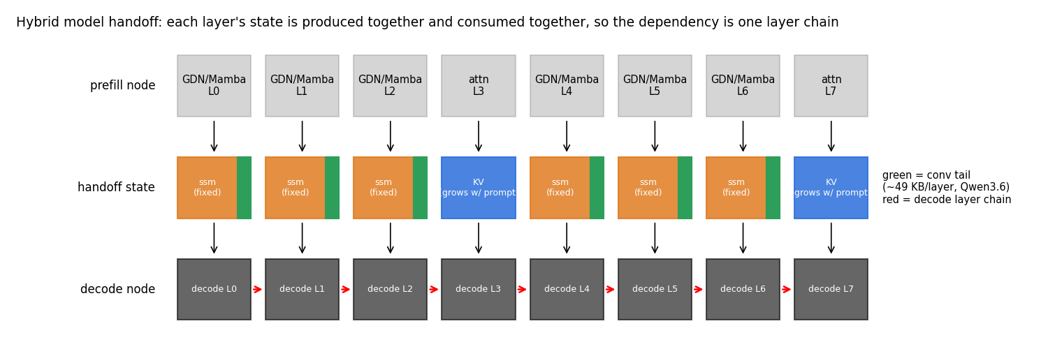
The same recurrent layer’s ssm and conv both serve one decode layer. The next layer still waits on that layer’s output. One narrow case remains. If conv arrives first and the runtime can split the work inside a layer, the convolution operator can start. The recurrent layer is still unfinished. A later layer still waits. Component-level readiness buys only a short head start inside the layer.
Arrived, runnable, and admitted are different events
A PD handoff has a data path and a compute path. The producer has to know when a layer’s state can be sent. The consumer has to know when the bytes on hand are enough for the next piece of compute. The scheduler still decides when the request may enter a batch.
vLLM’s disaggregated-prefill connector stores and loads state with the attention module, layer by layer. save_kv_layer is the producer’s per-layer send point. wait_for_layer_load is the consumer’s per-layer wait (vLLM disaggregated prefill). LMCache stores and moves KV. A layer-wise integration can overlap the load with compute (LMCache). Per-layer streaming already has an interface. NIXL moves bytes point to point across memory and storage backends (NIXL). A transport library moves bytes. When a transfer counts as done, which pieces are waited on, and which request may run, stay with the layer above. The library in use leaves the readiness granularity open.
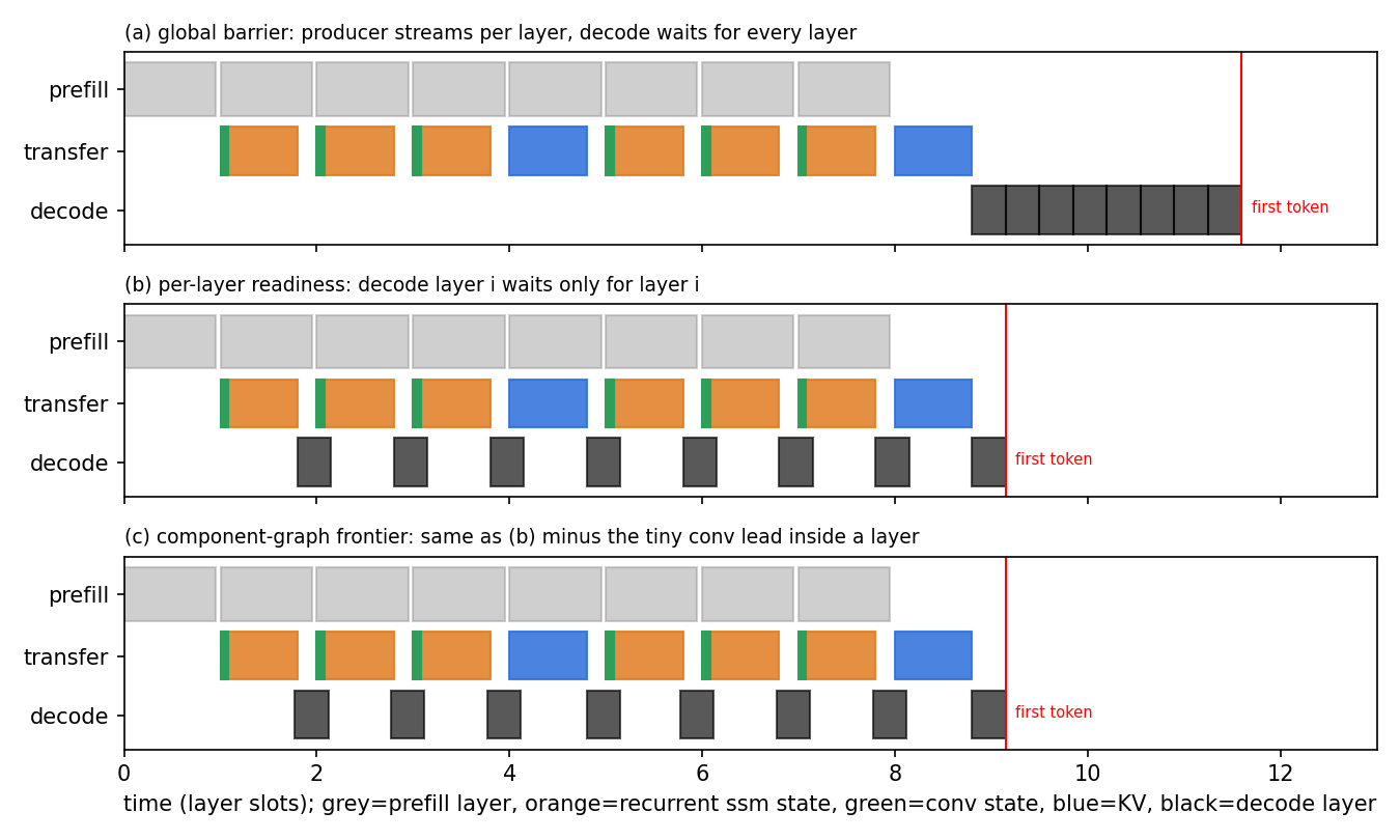
Removing the whole-request barrier releases several layers of compute. Splitting components inside a layer pays only when those components arrive apart, and when an operator can run on the piece that arrived. Figure 2 sketches that mechanism. Later figures carry the model latencies. Overlap differs by workload.
TL;DR
The question is whether a hybrid-model handoff needs a dependency graph finer than the layer. On a single-request model, component readiness beats layer readiness by at most 0.053%. The heavier sweep has 648 deterministic replay points. It covers speculative decoding, continuous batching, interleaved requests, and pipeline parallelism. The maximum there is still 1.98%. Every concrete workload’s median is 0.00%. Layer readiness against a global wait reaches 47.5%.
All of these are model values. The gain depends on whether the consumer has independent work it can start, and on whether the scheduler allows that work to run. More components do not by themselves mean more usable parallelism.
The hypothesis
The component story is specific. Put KV, ssm, and conv on a directed acyclic graph. Run a node as soon as its dependencies are met. That should release more compute than ordinary per-layer readiness. The ready frontier is the set of nodes whose dependencies are already satisfied.
The increment that matters is component-level against layer-level. Per-layer streaming can take the same gain over a global wait, so a win against global wait leaves the component question open. A 15% latency drop is the line used here for a gain worth caring about. The comparison uses the whole distribution.
A single-request layer chain is a weak test. The stronger test is a heavier workload. Speculative decoding adds a draft and a target. Continuous batching runs many requests together. Interleaving shares one link across requests. Pipeline parallelism cuts the model across devices. The question is whether those change what the consumer depends on, or only how the same chain queues and where it is placed.
Same bytes, different waits
The model covers Qwen3.6-35B-A3B and Nemotron-3-Nano-30B-A3B. Prompts are 1k, 8k, and 32k. Links are PCIe Gen4, 100G, and 25G. PCIe Gen4 bandwidth is a measured input. The handoff delays and the policy gains computed from it are still model outputs.
Prefill model FLOPs utilization, MFU, is 0.4 or 1.0. The first is a lower efficiency. The second is idealized. Two timings stay apart. Handoff may send while prefill is still computing. Migration starts the move only after compute finishes. Their overlap differs, so they stay separate configurations.
The four policies share the same bytes and the same compute. A finishes compute, then moves state. B is the stronger global-wait baseline. When streaming is allowed, the producer already sends layer by layer, and the consumer waits for every piece. C is ready per request and per layer. A decode layer waits for that layer’s state and for its compute predecessor. D splits the components inside C, and may run the part of the layer whose inputs have arrived.
The single-request sweep is 108 configurations and 216 comparisons. The event-graph sweep over four workload families is 648 replay points. A gain is the latency drop against the named baseline. Boxes and points are differences across configurations. Read them as configuration spread. Run-to-run noise and confidence intervals are outside this sweep.
The model takes a prefill MFU, an attention shape, a convolution operator share of 10%, and 0.05 ms to move an activation between pipeline stages. Request-level asynchronous execution assumes zero interference, and it leaves out the extra weight reads from splitting a batch. Semantic correctness of the schedule sits outside this model.
Short prompts still move a fixed state
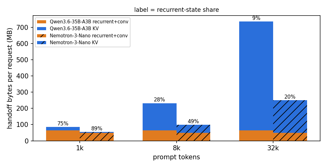
A shorter prompt leaves the recurrent state the same size. That fixed state is a floor under the transfer, so a short request can still pay a real move. At long prompts the recurrent share falls because KV grows. Attention keeps a KV entry per past token. A recurrent layer compresses history into a fixed shape. The orange bars stay nearly flat. The blue bars grow. That mix is why a short prompt on a slow link is where streaming matters. Bytes set how long the move takes. The consumer’s dependencies set what can run during the move. A pure attention model has no recurrent floor. Partial reuse would change which bytes move. The share of recurrent bytes and the share of end-to-end latency are different quantities.
The single-request gain is the layer stream
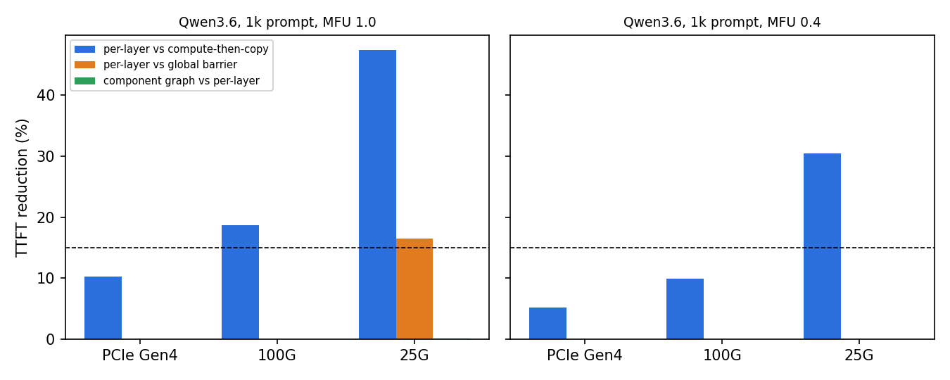
On 25G, per-layer readiness beats compute-then-move by up to 47%, and still by 31% at MFU 0.4. Against a global wait whose producer already streams, only the MFU 1.0 and 25G point clears 15%, at 16.5%. At MFU 0.4 that increment is 0. Component against layer improves by at most 0.053%. That is why the green bars are almost absent. Moving from compute-then-move to per-layer streaming opens overlap on both sides. Producer compute overlaps the transfer, and consumer compute overlaps it too. The global-wait baseline has already taken the producer half. What remains is idle time on the consumer. The tall blue bars are the layer stream.
conv and ssm of one layer come from the same prefill layer. Even if the convolution tail is sent first, decode can run only the convolution. It still needs the recurrent state to finish the layer. Qwen3.6’s convolution tail is about 49 KB per layer. On 25G that lead is about 16 µs. The overlap window is that arrival gap. The volume of the recurrent state is a different quantity. This is a single-request layer chain. 0.053% is the maximum increment in these configurations. When producer and consumer are both organized by layer, a component signal adds little beyond per-layer streaming.
Four workloads do not widen the per-request frontier
Speculative decoding drafts candidate tokens and has the target model check them, so fewer expensive serial steps are needed (vLLM speculative decoding). The model here is one draft layer and a candidate length k=3. That is the setting, and other speculative algorithms sit outside it. Continuous batching puts active requests in one decode step and updates the set on the step boundary. Interleaving is about how requests share the state link. Pipeline parallelism, PP, places layers on different devices and forwards activations.
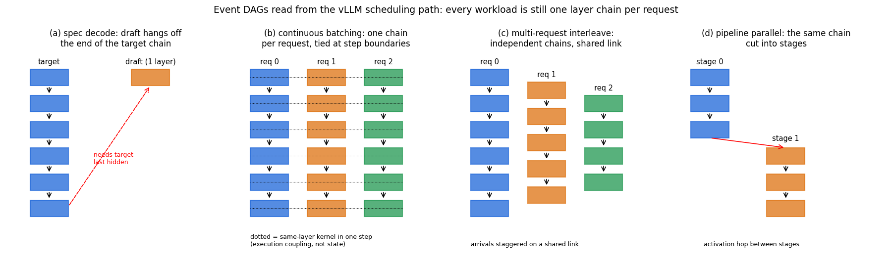
In the speculative panel, the modeled draft depends on the target’s last hidden state, so it hangs off the end of the target chain. The extra model role stays off the target’s handoff path. In the continuous-batch panel, dashed lines are requests sharing one GPU operator for a layer. The requests keep separate state. The runtime still binds them, which is why a whole batch can stall together. In the interleaved panel each request keeps its own layer chain. A shared link changes arrival order. The PP panel cuts one chain across devices and adds an activation hop. The later stage still needs the earlier stage’s output. Contention and cross-device traffic move the timeline. Components of one layer stay consumed together. Tree speculation, EAGLE-3’s multi-layer features, chunked prefill, and a partial handoff after a prefix-cache hit are outside this figure.
Layer streaming takes the large gains
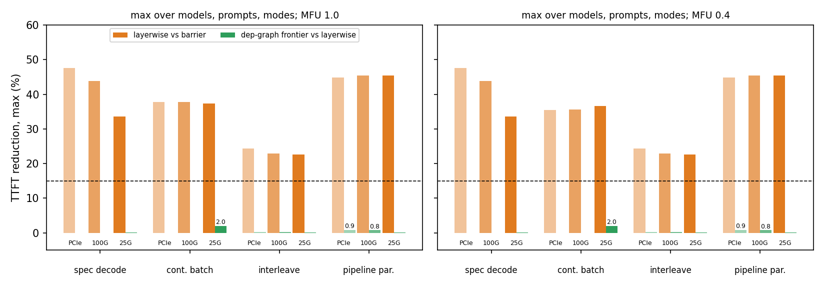
Per-layer readiness improves speculative decoding by up to 47.5%, continuous batching by about 37% to 38%, interleaving by about 23% to 24%, and PP by about 45%. The component increment tops out near 2.0%, on continuous batching at 25G. PP is about 0.8% to 0.9%. The rest sits near 0. Heavier workloads widen some gaps. The wide gap is still whether the consumer may run layer by layer. Splitting that chance into components inside a layer adds almost nothing. A global wait holds runnable compute behind one all-done event. Per-layer readiness releases it. The component frontier remains the per-request layer chain. MFU 0.4 and 1.0 look alike, so the small component increment is common to both efficiencies. Each bar is a group maximum, and the maxima need not share one configuration. The 47.5% is layer streaming on speculative decoding. It stays separate from the component graph.
Across the distribution, the component frontier stays flat
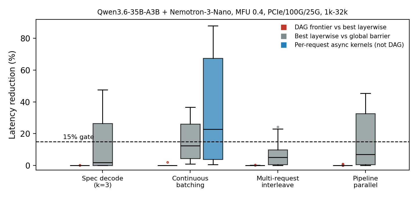
On continuous batching the gray median is about 12% and the maximum about 37%. Blue is request-level async execution. On that family its median is about 23% and its maximum is 88%. State can be ready while the request is still waiting to run. The blue box is execution freedom. An independent request need not wait out the original batch. That freedom and a finer state graph are different questions. Component readiness changes how a layer’s pieces are waited on. Request-level async changes how requests are bound together. The second one touches the step boundary and the shared operator, so it can move a longer wait. 88% is an upper bound under zero interference. The bound leaves out the extra weight traffic of a split batch. Splitting a batch changes utilization, memory traffic, and launch cost. The boxes are sensitivity across configurations.
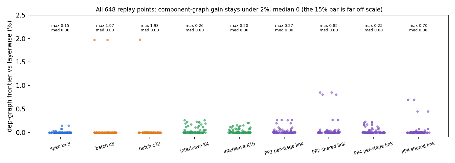
Across all 648 points the median of every group is 0.00%. The speculative maximum is 0.15%. Batch sizes 8 and 32 reach 1.97% and 1.98%. Interleaving at 4 and 16 reaches 0.26% and 0.20%. PP2 is 0.27% on a private link and 0.85% on a shared link. PP4 is 0.23% and 0.70%. A small change in arrival time can push a request across an execution boundary, so a few points leave zero. The 1.98% maximum sits on that kind of threshold. Reading it as general component parallelism of that size would stretch one boundary effect. Give the per-layer policy the same request-level async freedom, and the gap between the two is at most 0.34%. A fair comparison has to match both the readiness rule and the right to run. The result is for the models and schedulers in this sweep.
The step boundary is the wait that moves
A new request in continuous batching usually cannot join a step that is already running. Even if its state has arrived, it waits for the next admission point and then does its own compute. Discrete steps turn a continuous arrival into a whole-step wait. If the arrival phase is roughly uniform and a batched decode step takes D_c, the expected time from state-complete to the end of an execution step is about D_c/2 plus D_c. The first term is the wait for the boundary. The second is the step itself. In the model D_c is about 23 to 38 ms. A 1k transfer is about 7 to 27 ms. The scheduler boundary can already outweigh the transfer.
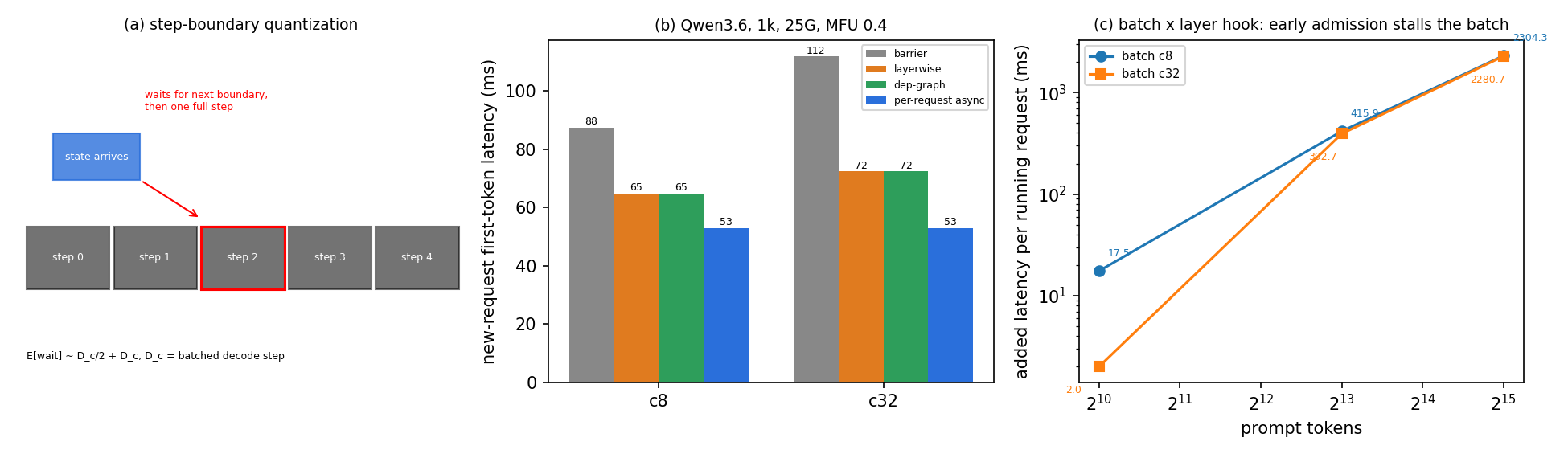
The center panel is Qwen3.6, 1k, 25G, MFU 0.4, handoff. For batch sizes 8 and 32, global wait is 88 ms and 112 ms. Per-layer readiness is 65 ms and 72 ms. Per-component readiness is still 65 ms and 72 ms. Request-level async execution is 53 ms and 53 ms. Finer components save nothing in this example. Async execution recovers 12 to 19 ms, and that recovery is the step-boundary quantization. While the request sits on an admission instant, a more precise state signal leaves the GPU on the same schedule. Shortening that wait means changing when a request may join, and how it runs with the others.
The right panel is the other failure. Admitting too early can hold the requests already running. In the vLLM per-layer hook modeled here, wait_for_layer_load waits on the whole batch and a layer name. Other requests in the batch have no bypass. Put a request that is still handing off into the batch. When execution reaches that layer, the whole batch can block on it. At 1k the extra delay is 17.5 ms at batch 8 and 2.0 ms at batch 32. At 8k it is about 0.39 to 0.42 seconds. At 32k it is about 2.28 to 2.30 seconds. At a long prompt the delay approaches the prefill itself. The consumer is waiting for state the producer has not created yet, on top of bytes already in flight. A per-layer signal should let useful compute proceed, and one unready request should stay off the batch’s wait condition. The hook modeled here hangs only on attention layers. GDN and Mamba layers have no matching hook. A per-layer KV interface covers KV. The other hybrid handoff states are separate. The right panel follows from the hook and from the admission assumption. It is a model of that hook. Request-level admission changes the behavior. A real async gain also pays for splitting the batch and for contention.
The consumer chain sets the gain
The opening question comes from the state mix. A hybrid model hands off KV, a recurrent state, and a convolution tail, so a component graph looks natural. In the models and four workloads covered here, each request still advances along a layer chain. Components of one layer are produced together and consumed together. Splitting them leaves a narrow frontier.
The gains that show up are per-layer streaming against a global wait, and the scheduling room that appears once requests may run apart. Those answer layer-to-layer waiting and request-to-request binding. Component granularity is a separate increment.
Every number is a deterministic model output. Semantic correctness sits outside this model. Prefill efficiency, attention shape, the draft, and pipeline transfer are assumptions. Raising the convolution operator’s share from 10% to 50% still leaves the component increment bounded by how far ahead the convolution state arrives. Multi-layer feature dependencies, tree speculation, and a partial handoff sit outside the model. The conclusion stays inside the cases above.
What a finer ready signal can and cannot buy
The value of a finer ready signal is set by what the consumer depends on. If components are produced together and merged by one consumer, a split completion signal can use only the real gap between their arrivals. Extra kinds of state become extra runnable work only when that gap is real.
A handoff optimization has to keep the overlap the system already has inside the baseline. Compute-then-move, a global wait with a streaming producer, and per-layer readiness are different increments. If the producer can send early, that ability stays in the baseline when a finer mechanism is judged. Leave it out, and the gain lands on the wrong change.
More requests and more devices add coupling. One request’s dependency frontier is a separate question. A shared operator, a shared link, and a pipeline cut all move where the wait sits. Whether state can be consumed early is still a data dependence, checked edge by edge.
After the data is ready, the scheduler’s quantization can be the larger wait. In the continuous-batch model the step and the transfer are the same order of time, and the ideal gain of request-level async execution is much larger than the component split. Admission that happens only on a discrete boundary has to be counted apart from state wait and from compute. The async upper bound also has to be kept apart from the cost of splitting the batch.
The scope of a wait hook is part of the performance semantics. If a per-layer wait blocks the whole batch, one unready request passes the producer’s delay on to requests that were already running. The bytes being waited on are one question. Who else waits, and whether every state type has a hook, are the next ones.
Related analysis
RL Long Tail: Mid-Batch Parallel Shape Switching asks whether an RL rollout should change parallel shape in the middle of the batch. It does not measure a prefill/decode split. This post starts after that split already exists, and asks how fine the handoff’s ready signal has to be.
状态可以拆得很细。能提前执行多少,取决于消费端的依赖链和调度边界。在确定性模型里,按组件等待相对按层等待最多改善 1.98%,每一类负载的中位数都是 0。按层等待相对等整次传输完成,最多改善 47.5%。
从状态搬运到计算就绪
大语言模型推理有两种计算形状。prefill 处理输入 prompt,建立后面生成要用的状态。decode 复用这些状态,逐步生成 token。prefill/decode 分离,简称 PD 分离,把两部分放到不同 GPU 上。两边可以各自配置资源,互相干扰也更少。
DistServe 按首 token 延迟和后续 token 间隔,为两边分别选资源和并行策略。交接带宽算在放置里(Zhong et al. 2024, OSDI)。Splitwise 从 prompt 计算和 token 生成在计算、内存、功耗上的差别出发。两边可以用不同硬件,中间状态经互连搬走(Patel et al. 2024, ISCA)。分离换来放置自由,也留下一个问题。decode 要等到多少状态,才开始有用的计算?
attention 层交接的是 KV cache,也就是历史 token 的 key 和 value。它随 prompt 变长。hybrid 模型把 attention 和线性递归层放在一起,状态就比 KV 多。GDN(Gated DeltaNet)或 Mamba 一类递归层,保留固定大小的递归态,以及短卷积窗口的尾部。下文 ssm 指递归态,conv 指卷积态。这两个名字只给交接组件分类。模型是否共用一套递推,要另看。
同一递归层产出的 ssm 和 conv,最后服务于同一个 decode 层。后续层还要等这个层的输出。有一个很窄的例外。conv 先到,而且执行系统允许拆开层内计算时,卷积子算子可以先启动。整个递归层这时还没完成。后续层仍要等。组件级就绪拿到的,是层内的一小段提前量。
搬到了、层能跑了、请求能跑了,是不同的事件
PD 交接要同时安排数据路径和计算路径。生产端要知道某层状态何时可以发送。消费端要知道手上的字节何时够做下一段计算。调度器还要决定请求何时进入执行批次。
vLLM 的 disaggregated prefill 把状态传输交给 connector,和 attention 模块一起按层存取。save_kv_layer 是生产端逐层保存或发送的时机。wait_for_layer_load 是消费端等待对应层的时机(vLLM disaggregated prefill)。LMCache 管理、存储和传输 KV。按层集成可以让加载和计算交错(LMCache)。按层流式已经有接口。NIXL 做点对点传输,并抽象不同的内存和存储后端(NIXL)。传输库负责搬字节。一次传输何时算完成、等哪些片段、哪个请求可以跑,仍由上层决定。用了哪一个库,就绪粒度仍是开放的。
去掉整个请求的等待屏障,可以释放多个层的计算。再拆同层组件,只有组件到达之间真有空隙,而且有独立子算子能跑,才有收益。图 2 画的是这个机制。后面的延迟来自模型。不同负载的可重叠时间各不相同。
TL;DR
要检验的问题是,hybrid 模型的状态交接要不要比层更细的依赖图。单请求模型里,组件级相对按层最多改善 0.053%。更重的一轮有 648 个确定性回放点,覆盖投机解码、连续批处理、多请求交错和流水线并行。最大值仍是 1.98%。每一类负载的中位数都是 0.00%。按层就绪相对全局等待,最多改善 47.5%。
这些都是模型值。决定收益的是消费端有没有独立计算可以提前执行,以及调度器是否允许执行。组件更多,并不自动意味着可用的并行更多。
假设
组件级方案可以讲得很具体。把 KV、ssm、conv 做成有向无环图里的节点。依赖一满足就推进。这样应当比普通按层就绪释放更多计算。就绪前沿就是当前依赖已经满足、可以执行的节点。
真正要看的增量,在组件级和按层之间。按层流式相对全局等待也能拿到同一笔重叠。组件级相对按层的问题还在。本文把 15% 的延迟降幅当作值得关心的线,比较用的是整段分布。
单请求层链对这个假设是弱检验。更强的检验来自更重的负载。投机解码加上 draft 和 target。连续批处理把多个请求放在一起跑。多请求交错让不同请求共用一条链路。流水线并行把模型切到不同设备。要问的是,这些改的是消费依赖,还是只改了同一条链怎么排队、放在哪里。
固定状态与计算,只改变等待方式
确定性模型覆盖 Qwen3.6-35B-A3B 和 Nemotron-3-Nano-30B-A3B。prompt 取 1k、8k、32k。链路取 PCIe Gen4、100G 和 25G。PCIe Gen4 的带宽是测量值。由此算出的交接延迟和策略收益仍是模型输出。
prefill 的模型浮点运算利用率 MFU 取 0.4 和 1.0。前者是较低的计算效率,后者是理想化效率。两种时机分开。handoff 允许 prefill 边算边送。migration 等计算结束才开始搬。重叠不同,所以两者是分开的配置。
四种策略用同一份字节、同一份计算。A 先算完,再搬状态。B 是较强的全局等待基线。允许边算边送时,生产端已经逐层发送,消费端等全部状态。C 按请求、按层判断就绪。decode 某一层只等该层状态和它的计算前驱。D 在 C 里面再拆组件。输入已经到齐的那一段可以先跑。
单请求分析有 108 个配置、216 个对比点。四类负载的事件图有 648 个回放点。收益是相对所比基线的延迟降幅。箱线和散点是配置之间的差异,按配置散布来读。重复运行的噪声和置信区间不在这轮里。
模型取了 prefill MFU、attention 形状、卷积子算子占比 10%,以及流水线段间激活传输 0.05 ms。请求级异步执行假定零干扰,并略去拆批带来的重复读权重。调度在语义上是否正确,在这个模型外面。
短 prompt 仍要搬一份固定状态
prompt 变短,递归态的大小不变。这份固定状态是交接字节的底座,所以短请求仍可能付一笔明显的搬运。长 prompt 下递归态占比下降,是因为 KV 变大了。attention 按历史 token 留 KV。递归层把历史压进固定形状。橙色几乎不随长度变,蓝色随长度涨。所以短 prompt、慢链路,是流式交接值得看的地方。字节决定要搬多久。消费依赖决定搬运期间能做什么。纯 attention 模型没有这份底座。有部分复用时,要搬的字节会变。递归态占交接字节的比例,和它占端到端延迟的比例,是两件事。
单请求上的大收益来自按层流式
25G 上,按层就绪相对先算后搬最多改善 47%,MFU 0.4 时仍有 31%。相对生产端已经在流式发送的全局等待,只有 MFU 1.0、25G 的点超过 15%,达到 16.5%。MFU 0.4 时这一增量为 0。组件级相对按层最多改善 0.053%。绿色柱因此几乎看不见。从先算后搬改成按层流式,两边的重叠一起打开。生产端计算和传输重叠,消费端计算和传输也重叠。全局等待基线已经拿走前一半。剩下能回收的,是消费端的空闲。高的蓝色柱来自按层流式。
同层的 conv 和 ssm 由同一个 prefill 层产出。即便先传卷积态,decode 也只能先做卷积。做完这一层仍要递归态。Qwen3.6 的卷积尾巴约 49 KB 每层。25G 上对应的领先约 16 µs。可重叠的窗口是这个到达差。整层递归态的体积是另一回事。这里是单请求层链。0.053% 是这些配置里的最大增量。生产和消费都按层组织时,组件级信号在按层流式之外多出来的很少。
四类负载没有加宽单请求的依赖前沿
投机解码先生成候选 token,再由 target 模型验证,用来减少串行生成里昂贵的执行(vLLM speculative decoding)。本文建模的是单层 draft、候选长度 k=3。其他投机算法在这个设定之外。连续批处理把活跃请求放进同一个 decode 步,并在步边界更新请求集合。多请求交错看不同请求如何共用状态传输链路。流水线并行,简称 PP,把模型层分到不同设备,前一段的激活传给后一段。
投机解码里,所建模的 draft 依赖 target 最后的隐藏状态,所以挂在 target 层链的末端。多出来的模型角色停在 target 交接路径之外。连续批处理里的横向虚线,是多个请求共用同层 GPU 算子。请求的状态仍然分开。执行系统把它们绑在一起,所以整批可以一起停。多请求交错里,各请求仍有自己的层链。共享链路改变的是到达顺序。PP 把一条链切到不同设备,段间多一次激活传递。后一段仍要前一段的输出。资源竞争和跨设备通信会挪动时间线。同层组件仍一起被消费。树状投机、EAGLE-3 的多层特征依赖、分块 prefill,以及前缀缓存命中后的部分交接,都在这张图外面。
大的收益在按层流式
按层就绪在投机解码里最多改善 47.5%,连续批处理约 37% 到 38%,多请求交错约 23% 到 24%,PP 约 45%。组件级增量最高约 2.0%,出现在连续批处理的 25G 配置。PP 约 0.8% 到 0.9%,其余接近 0。负载更重,有些差距会拉开。大的差距仍是消费端能不能逐层跑。后面层的状态还没到时,前面层已经可以推进。把这个机会再拆到同层组件,多出来的很少。全局等待把已经能跑的计算挡在一次全部完成之后。按层就绪把这层限制放开。组件前沿仍是每条请求自己的层链。MFU 0.4 和 1.0 的图形接近,所以组件增量很小,两档效率都如此。每根柱子是组内最大值,这些最大值不必来自同一个配置。47.5% 是投机解码上的按层流式。它和组件依赖图是分开的。
看分布,组件前沿没有稳定优势
连续批处理上,灰色中位数约 12%,最大约 37%。蓝色是请求级异步执行。这一类里中位数约 23%,最大 88%。状态已经够用时,请求仍可能在等执行。蓝色是执行自由。独立请求不必跟原批次一起等到结束。这份自由,和状态图细不细,是两个问题。组件级改的是同层片段怎么等。请求级异步改的是请求之间怎么绑。后者碰到步边界和共用算子,所以能挪动更长的等待。88% 是零干扰假设下的上界。拆批之后多出来的读权重没有算进去。拆批会改变 GPU 利用率、内存访问和启动开销。箱线图是配置敏感性。
全部 648 个回放点里,每组中位数都是 0.00%。投机解码最大 0.15%。批大小 8 和 32 分别是 1.97% 和 1.98%。交错 4 和 16 分别是 0.26% 和 0.20%。PP2 在独立链路和共享链路上分别是 0.27% 和 0.85%。PP4 分别是 0.23% 和 0.70%。执行有边界时,很小的到达变化就可能让请求赶上另一次执行机会,于是出现离开零的孤立点。最大的 1.98% 就在这种阈值附近。把它读成同等规模的普遍组件并行,会放大一个边界效应。再给按层策略同样的请求级异步自由,两者差距最多 0.34%。公平比较要同时对齐就绪规则和执行权。这个结果属于本轮里的模型和调度器。
真正突出的等待是执行步边界
连续批处理的新请求通常不能在一个正在执行的步中间加入。即使状态已经到齐,也要等下一个准入边界,再做自己的计算。离散的步把连续的到达量化成了整步等待。如果到达相位近似均匀,带批 decode 步长为 D_c,从状态到齐到做完一个执行步的期望时间,大约是 D_c/2 再加上 D_c。前一项是等下一个边界,后一项是执行本身。模型里 D_c 约为 23 到 38 ms。1k prompt 的传输时间约为 7 到 27 ms。这时调度边界已经足以比传输更显著。
中图固定 Qwen3.6、1k、25G、MFU 0.4、handoff。批大小 8 和 32 上,全局等待分别是 88 ms 和 112 ms。按层就绪是 65 ms 和 72 ms。组件级就绪仍是 65 ms 和 72 ms。请求级异步执行是 53 ms 和 53 ms。这个例子里,把组件拆得更细没有省时间。异步执行收回的 12 到 19 ms,来自步边界的量化。请求停在准入时刻上时,更精确的状态信号仍让 GPU 按原日程跑。要缩短这段等待,得改请求何时加入,以及它怎样和已有请求一起跑。
右图是另一头的问题。准入太早,会拖住已经在跑的请求。本文分析的 vLLM 按层钩子里,wait_for_layer_load 按整批和层名等。批里其他请求没有旁路。把还在交接的请求放进批次,执行走到那一层,整批都可能被它堵住。1k 时,批大小 8 和 32 分别多 17.5 ms 和 2.0 ms。8k 时约 0.39 到 0.42 秒。32k 时约 2.28 到 2.30 秒。长 prompt 下,这个量级接近整个 prefill。消费端在等生产端还没产生的状态,已经发出的字节之外还有这一段。按层信号应让有用的计算往前走。一个还没就绪的请求,应留在整批的等待条件之外。本文分析的钩子只挂在 attention 层。GDN 和 Mamba 层没有对应挂点。按层 KV 接口覆盖的是 KV。其余 hybrid 交接状态是另一件事。右图跟着钩子语义和准入假设走。它是这个钩子的模型。请求级准入会改变这个行为。真实的异步收益还要付拆批和资源竞争的成本。
消费端的层链决定了还能提前多少
开头的问题来自状态组成。hybrid 模型同时交接 KV、递归态和卷积态,组件图看起来很自然。在本文覆盖的模型和四类负载里,每个请求仍沿层链往前走。同层组件一起产出,也一起被消费。拆开之后,前沿仍然很窄。
显出来的收益有两笔。一笔是按层流式相对全局等待释放的重叠。另一笔是请求可以分开跑之后露出来的调度空间。它们分别对应层与层之间的等待,以及请求与请求之间的绑定。组件粒度是另外一笔增量。
所有数字都是确定性模型的输出。语义是否正确在这个模型外面。prefill 效率、attention 形状、draft 结构和流水线传输都是假设。即便把卷积子算子占比从 10% 放到 50%,这个结构里组件级增量仍受卷积状态到达领先量约束。多层特征依赖、树状投机和部分交接在模型外面。上面的结论停在已经覆盖的情形里。
更细的就绪信号能买到什么
就绪粒度值多少,由消费端依赖什么决定。组件一起产出,再由同一个消费单元合起来用,细化后的完成信号只能用它们之间真实的到达差。状态种类变多,只有这个到达差是真的,才多出可执行的工作。
评估交接优化时,系统已经有的重叠要留在基线里。先算后搬、生产端已经在流式发送的全局等待、按层就绪,是不同的增量。生产端能提前发送时,比较更细的机制仍要保留这个能力。把它拿掉,收益就会记到另一次改动上。
请求更多、设备更多,耦合会增加。单请求的依赖有没有变宽,是另一件事。批里共用的算子、共享的链路、流水线的切段,都会挪动等待的位置。状态能不能提前消费,仍是数据依赖,要逐条看。
数据就绪之后,调度的量化可能成为主要等待。连续批处理模型里,步长和传输时间处在可比较的量级。请求级异步执行的理想收益明显大于组件细化。准入落在离散边界上时,状态等待、准入等待和计算时间要分开算。异步方案的上界和拆批成本也要分开看。
等待钩子的作用域也是性能语义的一部分。按层等待如果堵住整批,一个还没就绪的请求就会把生产端的延迟传给已经在跑的请求。等的是哪一份字节,是一个问题。还有谁一起等,以及每种状态有没有挂点,是接下来的问题。
相关分析
RL 长尾上的并行形态切换 问的是 rollout 中途要不要换并行形态。它没有测 prefill 和 decode 分开。这一篇从分离已经存在之后问起,交接的就绪信号要细到组件,还是细到层就够了。