Logical Skew Is Not Physical Contention: How We Killed a Beautiful MoE Systems Idea Early
0. MoE communication in two figures
Before discussing the failed idea, it helps to be precise about what MoE actually communicates. In one MoE layer, the router does not compute the expert output; it selects a small set of experts for each token. Those experts run their MLPs, and their outputs are combined back at the token owner. MoE therefore creates a sparse token→expert dependency graph, not a dense all-to-all semantic dependency.
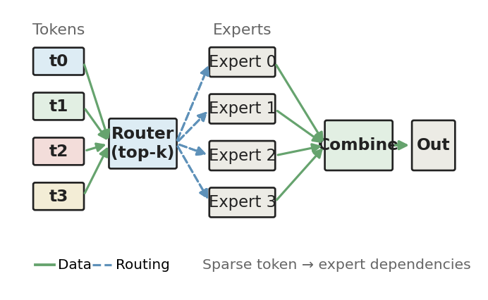
With Expert Parallelism (EP), experts are placed across GPUs. A token owned by one GPU may need to cross NVLink, PCIe, or RDMA to reach an expert on another GPU; the expert result then returns for combine. Every MoE layer therefore induces a dynamic source GPU → destination rank traffic matrix.
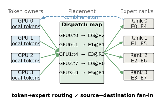
The subtle point—and the starting point of this story—is that the model’s “hot expert” graph and the network’s “how many independent sources converge on one physical receiver” graph are not the same graph. An expert may be hot while most of its tokens come from one source. A destination rank may host many distinct expert flows while still seeing only one or two senders.
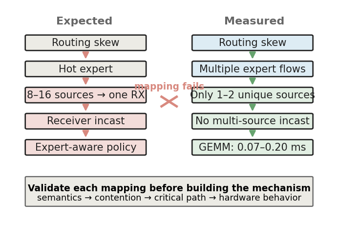
Our original IncastEP idea made a plausible but unverified jump exactly here: routing skew → hot expert → many-source incast. The rest of the blog is the story of how real workloads dismantled that chain one mapping at a time.
TL;DR. We started from a compelling hypothesis: skewed MoE routing should create
many sources → hot experttraffic, which should produce receiver-side incast; an expert-aware communication scheduler could then prioritize transfers that unlock useful computation and reduce MoE layer latency. The chain was elegant—but the workload did not cooperate. Across local EP=4 runs of GLM, Qwen, and Nemotron, both expert-level and destination-rank source fan-in stayed at p95=1 and max=2. Nemotron could stack many distinct expert flows on one destination, but they still came from only one or two source GPUs. Meanwhile, calibrated expert MLPs took only about 0.07–0.20 ms, leaving a much smaller “unlock compute early” window than our original synthetic setup suggested.We stopped before building credits, adaptive admission, or a custom kernel. The broader lesson is more useful than the abandoned design: before optimizing a bottleneck, validate three mappings—application semantics → physical resource contention, contention → critical-path delay, and experimental policy → actual hardware behavior.
1. Why the idea looked so plausible
MoE makes a seductive systems story. The router assigns tokens to experts, expert popularity is not perfectly uniform, and some experts become hotter than others. It is natural to imagine that a hot expert attracts traffic from many GPUs at once. At the network layer, that looks like classic many-to-one incast; at the model layer, the same hot expert can look like a compute straggler.
That gives a clean causal chain:
Routing skew
    ↓
Hot experts
    ↓
Many sources → one receiver
    ↓
Receiver-side incast
    ↓
Expert-aware communication scheduling
    ↓
Prioritize flows that unlock useful GEMM
    ↓
Lower MoE layer latency
It also suggests an attractive research tension: network-optimal need not be model-optimal. Suppose Expert A needs only four more tokens to launch its next useful GEMM chunk, while Expert B already has a full chunk waiting in its compute queue. A network-centric scheduler might prefer a larger transfer to B because it packs the link well or fits a matching objective. A model-progress scheduler might send A’s four tokens first, start useful compute earlier, and overlap it with the rest of the communication.
The reasoning is not logically wrong. The problem is that it silently crosses three unverified mappings:
- Does a hot expert actually imply many independent physical sources converging on one receiver?
- If arrival order changes, is the unlocked expert compute long enough to move the layer critical path?
- Does the experiment’s “different schedule” actually change what is launched on the wire?
Our experiments ended up falsifying—or at least sharply weakening—each assumption in turn.
2. First break: logical skew did not become multi-source physical incast
We eventually stopped looking only at “hot experts” and measured two distinct fan-in metrics.
For an expert e:
For a physical destination rank r:
The first is expert-level fan-in. The second is destination-rank fan-in. This distinction matters because low per-expert fan-in does not rule out physical contention: many different experts might be placed on the same rank or behind the same NIC, causing their traffic to converge again at the receiver.
We increased concurrency on GLM-4.7-Flash from 4 to 32, checked Qwen3.6-35B-A3B, and then used Nemotron-3-Nano at concurrency 32/64/128 as a stronger-expert and richer-flow case.
The result was stubbornly flat: expert fan-in p95=1, max=2; destination-rank fan-in p95=1, max=2. Increasing request concurrency did not push source cardinality toward the 8–16-source regime that the original IncastEP story implicitly relied on.
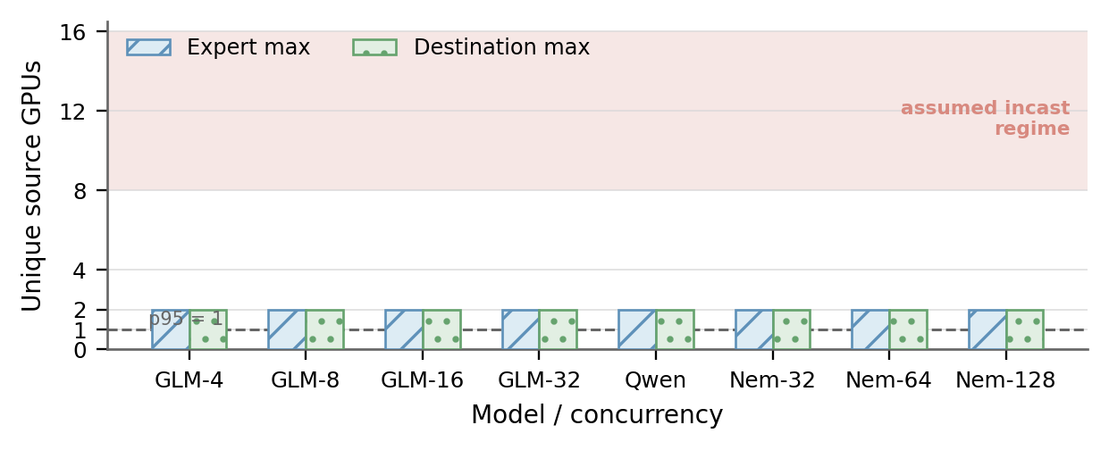
This became the most important negative result in the project. Under these local EP=4 configurations, the arrow
routing skew → many-source receiver incast
was simply not supported.
The subtle trap: many flows are not many sources
Nemotron made the distinction especially clear. At concurrency 128, a destination rank could see roughly p95=4, p99=12, and max=23 distinct expert flows. A message-count proxy reached about 30 in the tail. Looking only at the number of logical flows, the receiver appears busy and fragmented.
But plot those flow counts against the number of unique remote source GPUs for each (dispatch, destination rank):
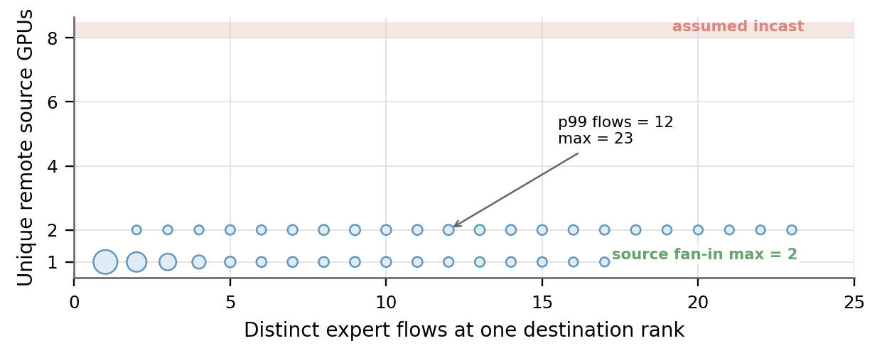
Almost the entire distribution sits on one or two sources.
A receiver can carry many semantically distinct expert flows without experiencing multi-source incast. Logical fragmentation is not physical fan-in.
That distinction is deeper than this one project. Models expose tokens, experts, top-k dependencies, and activation histograms. NICs expose endpoints, QPs, queues, bytes, and concurrent senders. Those are different graphs.
We do not have enough evidence to claim a universal reason for the persistent 1–2-source pattern. Fine-grained expert structure, token ownership, placement, and the serving runtime’s dispatch organization may all contribute. The important methodological point is not to invent a mechanism explanation after the fact. The measurement we can defend is narrower: the multi-source convergence assumed by our design did not appear in the configurations we measured.
3. Second lesson: a microbenchmark can make a bottleneck real without making it prevalent
Earlier synthetic experiments looked encouraging. In a cross-node, fixed-total-byte N→1 test at roughly 344 KiB offered traffic, increasing fan-in from 1 to 3 increased median network completion from roughly 0.29 ms to 0.81 ms.
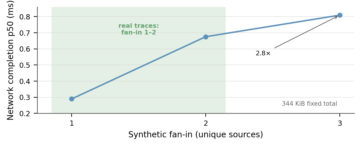
That observation was not wrong. If we force several sources to hit one receiver, multi-source contention can become a real network effect. But a microbenchmark answers a mechanism question, not a prevalence question.
The two responsibilities should be separated explicitly:
- Microbenchmarks establish causality: if fan-in increases, do arrival spread, receiver pressure, or completion time worsen?
- Workload characterization establishes prevalence: how often do real model executions actually enter that fan-in/flow-size regime?
Running only the first can produce a dangerous kind of paper: a system that successfully fixes a bottleneck that its benchmark manufactured.
One of the most useful process changes in this project was therefore to require controlled workloads to be calibrated from measured traces—source cardinality, flow sizes, expert mix, and compute cost—rather than designing a beautiful W1/W2 first and then searching for a workload that resembles it.
4. Third constraint: even a correct dependency may live on the wrong timescale
The original idea also relied on a second assumption: once an expert becomes ready earlier, its compute is long enough to overlap meaningful remaining communication and move the layer completion time.
Our first synthetic setup used large GEMMs, which made this easy to demonstrate. Calibrating the expert MLP with real model dimensions changed the picture.
On an A40:
- GLM-4.7-Flash was around 0.07 ms for 1–32 tokens and about 0.095 ms at 256 tokens;
- Nemotron-3-Nano was around 0.08 ms at small token counts and about 0.12 ms at 256;
- a DeepSeek-V4-Flash proxy calibration was around 0.11–0.12 ms for small batches and about 0.20 ms at 256 tokens.
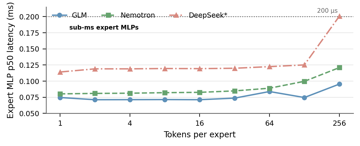
A useful first-order bound is:
\[\Delta T_{layer} \lesssim \min(T_{GEMM\ unlocked}, T_{comm\ remaining}) - T_{scheduling\ overhead}.\]If the expert compute itself is only 70–200 microseconds, the maximum useful overlap window is already small. Add admission logic, queue management, synchronization, or kernel-launch overhead, and a semantically correct scheduling improvement can quickly collapse into the noise floor.
The lesson is not that communication-compute overlap is useless. It is more precise:
Criticality in a dependency graph is not enough; the dependency must also have enough wall-clock budget to justify a separate mechanism.
This is why we stopped using inflated GEMMs as scientific evidence. If a scheduling idea requires multiplying the real expert compute time by ten to pass a Go threshold, we are validating the synthetic regime, not the original systems claim.
The DeepSeek-V4 serving trace itself was blocked by the current A40/vLLM FP8 KV-cache requirement, so the DeepSeek curve here is calibration-only, not end-to-end serving evidence.
5. A different kind of failure: our first negative experiment did not actually change the network schedule
One of the most useful lessons came from the experimental harness rather than the workload.
In the first W1 implementation, the receiver posted both irecvs up front and both senders immediately issued isend. What we called network_oracle and model_oracle mostly changed the receiver’s wait() order and when GEMM was launched.
We thought we were comparing:
Schedule A: flow 1 launches first, flow 2 later
Schedule B: flow 2 launches first, flow 1 later
but both flows were already live on the wire. We were comparing software observation order, not communication admission order.
Phase 2a fixed this with grant-before-isend. The receiver maintains an admission budget; a sender cannot issue the payload until it receives a grant. Only then can S_net=[2,1] and S_model=[1,2] produce genuinely different launch timelines.
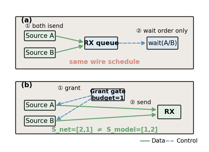
In a deliberately asymmetric harness-validation case, S_net=[2,1] achieved T_net≈0.410 ms, while S_model=[1,2] produced T_layer≈1.252 ms; the oracles disagreed, and the measured schedule gap was about 0.027 ms. But this case intentionally used highly asymmetric GEMMs (M=4096 vs M=8). It proved only one thing:
The harness can now instantiate two different physical schedules and can demonstrate that network and model objectives may disagree in a constructed case.
It did not prove that a useful disagreement exists in a real MoE workload.
This gives a broadly applicable experimental rule:
Before interpreting a negative result, verify that the two policies actually produce different physical execution at the system boundary.
For a network system, inspect grant/launch/packet timelines. For a GPU runtime, verify kernel order. For storage, verify the actual I/O path. A variable named network_oracle is not evidence that the network did something different.
6. The real lesson: validate three mappings before designing the mechanism
The IncastEP exploration can be compressed into three checks that are useful for almost any systems idea.
Mapping 1: application semantics → physical contention
Skew, hotness, sparsity, or dependencies at the model level do not automatically imply incast, queue buildup, or link imbalance at the network level.
Our concrete counterexample was:
many/hot expert flows
      ≠
many unique source GPUs
      ≠
receiver-side incast
Measure the endpoint-level traffic graph before designing the transport.
Mapping 2: physical contention → critical-path budget
Even if contention is real, ask whether it sits on the metric that matters and how many microseconds are actually recoverable.
Here, expert compute was often around 0.1 ms, so “make this expert ready earlier” had a very limited budget to turn into end-to-end layer latency.
Calibrate real compute and communication times before reasoning about overlap.
Mapping 3: experimental policy → actual hardware behavior
Changing a queue in software does not guarantee that the NIC saw a different schedule. Changing a wait order does not mean send order changed.
Every hypothesis test needs a sanity check that the policy actually changed the machine.
We now like to express this as a short pre-mechanism checklist:
1. Am I measuring a model-level metric or a physical-resource metric?
2. How much wall-clock critical-path budget does this physical effect occupy?
3. Do the compared policies actually differ on the wire/GPU/I/O path?
4. Does the synthetic stress regime fall inside the real workload distribution?
5. If the real workload does not enter that regime, am I willing to stop?
The fifth question is the hardest—and probably the most valuable.
7. Does this prove that MoE never has incast? No.
The result must be scoped carefully.
What the data supports is:
In the local EP=4 continuous-batch configurations we measured for GLM, Qwen, and Nemotron, we did not observe the strong multi-source expert/destination-rank incast required by the original IncastEP story.
It does not establish that:
- all MoE models avoid incast;
- EP=8/16, larger clusters, different token ownership, or different dispatchers behave the same way;
- coarse-grained 8/16-expert models cannot produce stronger fan-in;
- production-scale NIC congestion is absent;
- many small expert flows have no optimization opportunity.
We deliberately did not download Mixtral just to rescue the story. Cross-node EP=8 was skipped after the local destination-rank signal stayed flat. DeepSeek-V4 serving traces were blocked by current FP8 KV-cache support. And the message counts in our routing analysis are (src,dst,expert)-level proxies, not NIC hardware counters.
A useful negative result has value because its boundary is explicit, not because it is promoted into a universal theorem.
8. What became more interesting after the idea died?
Stopping IncastEP did not make the data useless. It exposed two questions that fit the measured workload better.
8.1 Token-ready, not expert-ready
With top-k routing, a token cannot enter combine until its required expert contributions are available. The most valuable transfer may therefore be the one that converts many tokens from “partial” to combine-ready, not the one that makes an expert receive a few more tokens.
A new scheduling question would be:
Which pending communication completes the most token dependencies on the critical path?
That is a token-level dependency problem, not an incast problem. It needs a fresh falsification step; it cannot inherit IncastEP’s motivation by assumption.
8.2 Many flows from few sources: fragmentation and coalescing
Nemotron showed p99≈12 and max≈23 distinct expert flows on a destination rank while source fan-in remained 1–2. That points toward a different communication cost model:
- launch/notification/completion overhead for many small expert messages;
- coalescing several expert flows on the same
src→dstpath and scattering at the receiver; - metadata and polling overhead that may dominate tiny payloads.
This is almost the opposite of the original design. Instead of throttling many senders, the right primitive may be to coalesce many semantic flows from the same sender.
The useful shift is that the workload is now telling us what mechanism to consider, instead of the mechanism telling us what workload to look for.
9. Stopping early is progress
The dangerous failure mode in systems research is not a null result. It is building months of mechanism before discovering that the motivation never existed in the workload.
We were fortunate to put workload characterization, GEMM calibration, and harness validation in front of credits, adaptive scheduling, and kernel work. The outcome was that we stopped.
That stop saved engineering time and left behind a more reusable principle than the original design:
Before optimizing a system bottleneck, verify application semantics → physical resource contention, contention → critical-path delay, and experimental policy → actual hardware behavior.
Or more plainly:
Do not infer network congestion from model skew, do not infer optimization value from DAG criticality, and do not infer hardware behavior from the names of two software policies.
A beautiful systems story is worth pursuing. A disciplined process that can kill it early is worth even more.
0. 先用两张图看懂 MoE 通信
在进入这次“失败的 idea”之前,先把 MoE 的通信对象说清楚。一个 MoE layer 里,Router 并不直接做计算,它只是为每个 token 选择少数几个 Expert。被选中的 Expert 分别执行 MLP,最后这些结果再回到 token 的 owner 做 combine。也就是说,MoE 天然产生的是一个稀疏的 token→Expert dependency graph,而不是所有 token 都访问所有 Expert。
当 Expert 被分布到多张 GPU 上时,这个逻辑依赖图就变成了 Expert Parallelism(EP)的通信。一个 source GPU 持有的 token 可能要跨 NVLink、PCIe 或 RDMA 发送到另一个 GPU 上的 Expert;Expert 算完后,结果还要回到原来的 token owner。每一层因此会生成一个动态的 source GPU → destination rank traffic matrix。
这里最容易混淆的一点,也是后面整个故事的起点,是:模型看到的“哪个 Expert 热”,和网络看到的“多少个独立 source 同时打向哪个 physical receiver”,并不是同一张图。 一个 Expert 可以很热,但这些 token 可能主要来自一个 source;反过来,一个 destination rank 可以承载很多不同 Expert flow,却仍然只对应一两个发送端。
我们最初的 IncastEP idea,恰恰是在这里做了一个看似自然但未经验证的跳跃:routing skew → hot expert → many-source incast。下面的实验复盘,就是看这条链是怎样被真实 workload 一层层拆掉的。
TL;DR:我们最初相信,MoE 的 Expert 路由倾斜会自然形成
many sources → hot expert的接收端 incast,因此可以用 Expert-aware 的通信调度来改善模型关键路径。这个故事很顺,但真实 workload 一层层把它拆掉了:在 GLM、Qwen、Nemotron 的本地 EP=4 实验中,Expert fan-in 和 destination-rank fan-in 的 p95 都是 1,max 只有 2;Nemotron 虽然一个目的端可以同时承载很多 Expert flow,但这些 flow 仍然只来自 1–2 个 source。与此同时,真实 Expert GEMM 只有约 0.07–0.20 ms,能靠“提前解锁计算”隐藏的窗口也比想象中小得多。最终我们没有继续写 credits、adaptive scheduler 或 kernel,而是停掉了 IncastEP framing。这篇文章不是一个“实验失败”的记录,而是一个更普适的 lesson:在开始优化之前,要先验证三层映射——模型语义是否真的变成物理资源竞争,物理竞争是否真的落在关键路径上,以及你的实验 policy 是否真的改变了硬件行为。
1. 为什么这个 Idea 一开始很有吸引力?
MoE 的直觉很容易让人走到这里:Router 会把不同 token 送到不同 Expert,而 Expert activation 通常并不均匀。如果某几个 Expert 变成热点,那么很多 GPU 似乎就会同时往同一个 Expert 所在的 GPU 发 token。对网络来说,这看起来像一个经典的 many-to-one incast;对模型执行来说,这个 hot Expert 又很可能成为 straggler。
于是一个非常自然的系统故事出现了:
Routing skew
    ↓
Hot Expert
    ↓
Many sources → one receiver
    ↓
Receiver-side incast
    ↓
Network scheduler should understand Expert progress
    ↓
Prioritize flows that unlock useful GEMM
    ↓
Lower MoE layer latency
它甚至还有一个很漂亮的理论冲突:“网络最优”不一定等于“模型最优”。 假设 Expert A 只差 4 个 token 就能启动下一块 GEMM,而 Expert B 已经积压了一整个可执行 chunk;从网络角度继续给 B 发一个大 flow 可能更容易填满链路,但从模型角度,先把 A 的 4 个 token 补齐可能更快地启动有效计算,并和剩余通信重叠。
这个故事的问题不是逻辑错误,而是它偷偷跨过了三层没有验证的映射:
- Hot Expert 是否真的意味着多个独立 source 同时打到一个 receiver?
- 即使 arrival order 不同,提前启动的 Expert compute 是否足够长,能影响 layer critical path?
- 我们写的“不同 schedule”是否真的改变了 wire 上的发送行为?
后面的实验,正好一层层回答了这三个问题。
2. 第一层断裂:Logical skew 并没有变成 multi-source physical incast
为了避免只看“哪个 Expert 热”,我们后来同时定义了两个 fan-in:
\[F_e = \left|\{s\mid \exists\ t\ \text{from source }s\text{ routed to expert }e\}\right|\]和
\[F_r = \left|\{s\mid \exists\ e\mapsto r,\ \text{source }s\text{ sends remote tokens to rank }r\}\right|.\]前者是 Expert-level fan-in,后者是 physical destination-rank fan-in。这是一个很重要的区分:即使每个 Expert 只有少数 source,也可能有很多不同 Expert 同时落到同一个 rank/NIC,从而在物理层重新聚合成 incast。
我们先在 GLM-4.7-Flash 上把 concurrency 从 4 提到 32,又检查了 Qwen3.6-35B-A3B;随后为了增加 Expert 计算量和 flow 丰富度,又跑了 Nemotron-3-Nano,concurrency 做到 32/64/128。
结果非常稳定:Expert fan-in p95=1、max=2;destination-rank fan-in 也是 p95=1、max=2。 concurrency 增加并没有把 source cardinality 推到原故事期待的 8–16。
这张图对我们来说是整个项目最重要的 negative result。它说明,至少在这些本地 EP=4 配置和 workload 下,“routing skew → many-source incast”这个箭头不能直接成立。
更容易误判的一点:Many flows ≠ many sources
Nemotron 的数据很有意思。concurrency=128 时,一个 destination rank 上的 distinct expert flows p95 约为 4、p99 约为 12、max 达到 23;message-count proxy 甚至 max≈30。只看“一个 receiver 上有多少逻辑 flow”,这很容易让人觉得网络压力应该已经很复杂。
但是把每个 (dispatch, destination rank) 的 flow 数和 unique remote source GPUs 画在一起,现象非常清楚:
绝大多数点都压在 1–2 sources 两条线上。也就是说:
一个 receiver 可以同时承载很多语义上不同的 Expert flow,但这些 flow 完全可能来自同一个或两个发送端。逻辑 fragmentation 不等于 multi-source incast。
这是这次探索里最值得保留下来的技术 insight 之一。网络瓶颈看的是物理 endpoint、并发 source、QP/NIC queue 和字节到达模式;模型看到的却是 token、Expert、top-k dependency。两者不是同一个图。
我们目前的数据并不能解释为什么所有模型都稳定落在 1–2 source——这与模型的 fine-grained expert structure、EP token ownership、placement 和 vLLM 的 dispatch 组织都可能有关。重要的是不要在没有证据时替这个现象编一个机制解释。 我们真正能说的是:在测到的这些配置里,原来预期的物理 many-source convergence 没出现。
3. 第二层断裂:Microbenchmark 能制造瓶颈,但不能证明 workload 会进入这个 regime
更早的 synthetic fan-in microbenchmark 其实给过我们一个“看起来不错”的信号。在跨节点固定总字节实验中,约 344 KiB 总流量下,fan-in 从 1 增加到 3 时,T_net p50 从约 0.29 ms 增长到约 0.81 ms。
这没有错。如果我们强行制造 N→1,多 source contention 确实可以变成一个真实的网络问题。 但它只能回答“这个机制在某个 regime 下是否存在”,不能回答“真实 workload 是否经常进入这个 regime”。
这两类实验的责任应该严格分开:
- Microbenchmark:回答因果关系和机制,例如增加 fan-in 是否增加 arrival span、receiver pressure 或 completion time。
- Workload characterization:回答 prevalence,也就是真实模型到底有多少次落入这个 fan-in/flow-size 区间。
如果只做前者,很容易写出一个“系统成功解决了自己制造的瓶颈”的论文。
这次项目最有价值的一个流程改动,就是开始要求 controlled workload 的参数必须由真实 trace 反推,而不是先设计一个漂亮的 W1/W2,再去寻找能够配合它的 workload。
4. 第三层约束:即使能提前解锁 Expert,时间尺度也可能不够
原始故事还有另一个隐含前提:一个 Expert 一旦提前 ready,就有足够长的 GEMM 可以和后续通信重叠,从而真正缩短 layer completion。
我们一开始用的 synthetic GEMM 尺寸非常大,这会让这个故事天然成立。后来把它替换成真实模型维度后,结果完全不同。
在 A40 上:
- GLM-4.7-Flash:1–32 tokens 约 0.07 ms,256 tokens 约 0.095 ms;
- Nemotron-3-Nano:小 batch 约 0.08 ms,256 tokens 约 0.12 ms;
- DeepSeek-V4-Flash 的 proxy calibration:小 batch 约 0.11–0.12 ms,256 tokens 约 0.20 ms。
一个很粗但很有用的上界是:
\[\Delta T_{layer} \lesssim \min(T_{GEMM\ unlocked},\ T_{comm\ remaining}) - T_{scheduling\ overhead}.\]当 T_GEMM 自身只有 0.07–0.20 ms 时,所谓“先让 Expert ready,再用计算隐藏通信”的理论 headroom 已经很小。如果调度、grant、queue management 或 kernel launch 再吃掉几十微秒,最终的可见收益很容易只剩噪声级别。
这里的 lesson 不是“compute-communication overlap 没价值”,而是:
任何 critical-path 优化都必须先做 timescale matching。一个 dependency 在 DAG 上很关键,并不意味着它在真实硬件时间尺度上值得单独优化。
这也是为什么我们后来明确禁止“为了过 Go gate 而人为增大 GEMM”。如果必须把 Expert compute 放大十倍才能证明 schedule 有用,那么证明的是 synthetic workload,而不是原来的系统问题。
DeepSeek-V4 的 serving dump 最终还因为当前 A40/vLLM 的 fp8 kv-cache 要求被阻塞,因此这里只把它当作 GEMM proxy calibration,不能把它写成真实 serving evidence。
5. 一个更隐蔽的失败:我们的第一版实验其实没有改变网络 schedule
这次探索里最值得反复提醒自己的 lesson,反而来自一个实验 harness bug。
最早的 W1 里,receiver 一开始把两个 irecv 都 post 了,两个 sender 也都立即 isend。所谓 network_oracle 和 model_oracle 的区别,实际上只是 receiver 先 wait() 哪个 request,以及什么时候启动 GEMM。
换句话说,我们以为在比较:
Schedule A: flow 1 first, flow 2 later
Schedule B: flow 2 first, flow 1 later
实际上 wire 上两个 flow 都已经启动了。我们比较的只是软件观察/等待顺序,不是网络 admission order。
后来 Phase 2a 把 harness 改成 grant-before-isend,receiver 维持一个 admission budget,sender 必须先拿到 grant 才能真正发送。这样 S_net=[2,1] 和 S_model=[1,2] 才会产生不同的 send-launch timeline。
在一个专门为了验证 harness 的 asymmetric unlock case 中,S_net=[2,1] 的 T_net≈0.410 ms,而 S_model=[1,2] 的 T_layer≈1.252 ms,两种 oracle 确实不同;但 Δ_schedule 只有约 0.027 ms,而且这个 case 故意用了非常不对称的 GEMM(M=4096 vs 8),所以它只能证明:
“网络最优和模型最优可以在某个构造出来的 workload 上不同”这个实验框架现在是真的。
它不能证明真实 MoE workload 里存在值得优化的 gap。
这也给出了一个非常通用的实验原则:
在解释负结果之前,先验证两个 policy 是否真的在系统边界上产生了不同的物理执行。
对网络系统来说,要看的是 packet/flow launch、grant、queue 或 wire timeline;对 GPU kernel 来说,要确认 kernel launch/order 真不同;对 storage 来说,要确认实际 IO path 真不同。否则“没有收益”可能只是因为两个实验 arm 根本是同一个世界。
6. 最终我们学到的不是“IncastEP 不行”,而是三个映射必须逐层验证
如果把这次探索抽象成一个方法论,我会用下面三个问题过滤几乎所有 systems idea。
Mapping 1:Application semantics → Physical contention
模型层面的 skew、hotness、dependency、sparsity,并不会自动变成网络层面的 incast、queue buildup 或 link imbalance。
这次最直接的例子就是:
Hot / many expert flows
    ≠
Many unique source GPUs
    ≠
Receiver-side incast
先测 endpoint-level traffic graph,再设计 transport。
Mapping 2:Physical contention → Critical-path budget
即使某个资源真的有 contention,也要问它是否落在用户关心的关键路径上,以及可优化窗口有多大。
这次 Expert MLP 只有约 0.1 ms,因此“提前 ready”即使在语义上正确,能转化成多少 layer latency 仍然是另一个问题。
先做真实 compute/network calibration,再讨论 overlap。
Mapping 3:Experimental policy → Actual hardware behavior
一个变量名叫 network_oracle 并不意味着它真的改变了网络;一个 scheduler 改了队列顺序,也不意味着 NIC 看到了不同的流量。
每个 hypothesis test 都应该有一个“policy actually changed the machine” sanity check。
这三个 mapping 可以变成一个非常简单的预实验 checklist:
1. 我看到的是模型层 metric,还是物理资源 metric?
2. 这个物理现象占关键路径多少微秒/毫秒?
3. 两个对照 policy 是否真的在 wire / GPU / IO path 上不同?
4. synthetic stress 的参数是否落在真实 workload 的分布里?
5. 如果真实 workload 不进入该 regime,我是否愿意停止,而不是继续造机制?
最后一条可能最难,但也最重要。
7. 这是不是说明 MoE 永远没有 incast?不是
我们必须非常克制地解释这个 negative result。
目前能支持的结论只有:
在我们测到的 GLM、Qwen 和 Nemotron 的本地 EP=4 continuous-batch 配置中,没有观察到原 IncastEP story 所依赖的强 multi-source Expert/destination-rank incast。
它不等于:
- 所有 MoE 模型都不会出现 incast;
- EP=8/16、更多节点、不同 token ownership 或不同 dispatcher 也不会出现;
- coarse-grained 8/16-expert MoE 不会出现;
- 更高规模的生产集群没有 NIC-level congestion;
- “many small Expert flows”本身没有通信优化空间。
我们没有为了救故事下载 Mixtral;跨节点 EP=8 在没有 destination-rank signal 后也停止了;DeepSeek-V4 serving trace 又被当前 FP8 KV-cache 支持阻塞。另一个限制是目前 message count 是从 (src,dst,expert) 聚合出来的 proxy,而不是 NIC hardware counter。
8. 哪些问题反而因为这次失败变得更有意思?
停止 IncastEP 并不意味着这些数据没有留下新的问题。相反,它把两个更贴近真实 workload 的方向暴露了出来。
8.1 Token-ready,而不是 Expert-ready
MoE 的 top-k token 需要等多个 Expert contribution 都完成才能 combine。真正重要的 flow 也许不是“让某个 Expert 多拿几个 token”,而是:
哪条通信完成后,会让最多 token 从 partial state 变成 combine-ready?
这把调度语义从 Expert progress 下沉成 token dependency progress。它是否有足够的 gap,需要重新做 falsification,不能从 IncastEP 自动推导。
8.2 Many flows from few sources:fragmentation / coalescing
Nemotron 的一个 destination rank 可以看到 p99≈12、max≈23 个 distinct Expert flows,却仍然只有 1–2 个 source。这不是 incast,但它可能是另一类问题:
- 多个小 Expert message 的 launch/notify/completion overhead;
- 同一
src→dst上能否跨 Expert coalesce,再在 receiver scatter; - flow-level metadata 和 kernel polling 是否比 payload 本身更贵。
这个问题和原来的“限制 many-source admission”几乎相反:不是 throttle,而可能是 coalesce。
重要的是,我们现在有真实数据告诉我们应该往哪里看,而不是从一个漂亮架构图反推 workload。
9. 结语:早点杀掉一个 Idea,也是一种进展
系统研究里最危险的状态,不是实验失败,而是已经写了很多机制之后才发现 motivation 不存在。IncastEP 这次相对幸运:我们先做了 workload characterization、GEMM calibration 和 harness validation,然后才决定要不要进入 credits / adaptive scheduling / kernel implementation。
结果是我们停了。
但这个“停”其实保存了大量时间,也留下了一个比原系统设计更可复用的经验:
Before optimizing a system bottleneck, verify three mappings: application semantics → physical resource contention, contention → critical-path delay, and experimental policy → actual hardware behavior.
翻成更直白的话:
不要因为模型上有 skew,就假设网络上有拥塞;不要因为 DAG 上有依赖,就假设它值得优化;也不要因为代码里有两个 policy 名字,就假设硬件真的执行了两个不同的世界。
漂亮的 systems story 值得追,但更值得建立一套能够尽早杀掉它的实验流程。